NBER WORKING PAPER SERIES
STEM CAREERS AND THE CHANGING SKILL REQUIREMENTS OF WORK
David J. Deming
Kadeem L. Noray
Working Paper 25065
http://www.nber.org/papers/w25065
NATIONAL BUREAU OF ECONOMIC RESEARCH
1050 Massachusetts Avenue
Cambridge, MA 02138
September 2018, Revised June 2019
Previously circulated as “STEM Careers and Technological Change.” Thanks to David Autor,
Pierre Azoulay, Jennifer Hunt, Kevin Lang, Larry Katz, Scott Stern, and seminar participants at
Georgetown, Harvard, University of Zurich, Brown, MIT Sloan, Burning Glass Technologies, the
NBER Labor Studies, Australia National University, University of New South Wales, University
of Michigan, University of Virginia and the Nordic Summer Institute in Labor Economics for
helpful comments. We also thank Bledi Taska and the staff at Burning Glass Technologies for
generously sharing their data, and Suchi Akmanchi for excellent research assistance. All errors
are our own. The views expressed herein are those of the authors and do not necessarily reflect
the views of the National Bureau of Economic Research.˛
NBER working papers are circulated for discussion and comment purposes. They have not been
peer-reviewed or been subject to the review by the NBER Board of Directors that accompanies
official NBER publications.
© 2018 by David J. Deming and Kadeem L. Noray. All rights reserved. Short sections of text, not
to exceed two paragraphs, may be quoted without explicit permission provided that full credit,
including © notice, is given to the source.

STEM Careers and the Changing Skill Requirements of Work
David J. Deming and Kadeem L. Noray
NBER Working Paper No. 25065
September 2018, Revised June 2019
JEL No. J24
ABSTRACT
Science, Technology, Engineering, and Math (STEM) jobs are a key contributor to economic
growth and national competitiveness. Yet STEM workers are perceived to be in short supply.
This paper shows that the “STEM shortage” phenomenon is explained by technological change,
which introduces new job skills and makes old ones obsolete. We find that the initially high
economic return to applied STEM degrees declines by more than 50 percent in the first decade of
working life. This coincides with a rapid exit of college graduates from STEM occupations.
Using detailed job vacancy data, we show that STEM jobs change especially quickly over time,
leading to flatter age-earnings profiles as the skills of older cohorts became obsolete. Our findings
highlight the importance of technology-specific skills in explaining life-cycle returns to
education, and show that STEM jobs are the leading edge of technology diffusion in the labor
market.
David J. Deming
Harvard Graduate School of Education
Gutman 411
Appian Way
Cambridge, MA 02138
and Harvard Kennedy School
and also NBER
Kadeem L. Noray
Harvard University
Appendix is available at http://www.nber.org/data-appendix/w25065

1 Introduction
A vast body of work in economics nds that technological change increases the relative
wages of educated workers by complementing their skills, leading to rising wage inequality
(e.g. Katz and Murphy 1992, Berman et al. 1994, Autor et al. 2003, Acemoglu and Autor
2011). Empirical conrmation of this skill-biased technological change (SBTC) hypothesis
comes from the increasing return to a college education, which is interpreted as a single-
index measure of worker skill.
1
Yet despite large dierences in the curricular content of
college majors and in returns to eld of study, there is little direct evidence linking changes
in skill demands to the specic human capital learned in school.
2
Simply put, the process by
which technology changes the returns to skills by altering job tasks remains mostly a “black
box”.
3
In this paper, we study the impact of changes in the skill content of work on the labor
market returns to a form of specic human capital—Science, Technology, Engineering, and
Math (STEM) degrees.
4
STEM careers are ideal for studying the link between technology
1
In the canonical skill-biased technological change (SBTC) framework, technological progress increases
the productivity of high-skilled workers more than low-skilled workers, and so the skill premium increases
when technological change “races ahead” of growth in the supply of skills (Tinbergen 1975, Goldin and Katz
2007). Acemoglu and Autor (2011) develop a task-based framework that allows for a more general type of
technological bias, and they show the replacement of routine “middle-skill” tasks by machines could lead to
polarization of the wage distribution. In both cases, however, there is a single index of skill, and technologies
are not linked to specic job tasks.
2
The SBTC literature cited above shows the impact of technological change on the returns to general
skills (e.g. a college education). There is also a large literature studying heterogeneity in returns to eld of
study (e.g. Arcidiacono 2004, Pavan 2011, Altonji, Blom and Meghir 2012, Carnevale et al. 2012, Kinsler and
Pavan 2015, Altonji, Arcidiacono and Maurel 2016, Kirkeboen et al. 2016 Few studies connect technological
change to changes in the returns to specic skills. One exception is the literature studying general versus
more vocational educational systems across countries, which generally nds that 1) youth in countries with
a more vocational focus have higher employment and earnings initially, but lower wage growth (Golsteyn
and Stenberg 2017, Hanushek et al. 2017); and 2) that individual dierences in the returns to general
vs. vocational education are near zero for the marginal student, with observable dierences due mostly to
selection (Malamud 2010, Malamud and Pop-Eleches 2010).
3
“Insider econometrics” studies within rms show that technology adoption favors skilled workers, while
also having specic, non-neutral impacts on jobs that vary in their task content and specic skill requirements
(e.g. Autor et al. 2002, Bresnahan et al. 2002, Bartel et al. 2007, Ichniowski and Shaw 2009)
4
Field of study is an important mediator for understanding the returns to education. Lemieux (2014)
estimates that occupational choice and matching to eld of study can explain about half of the total return
to a college degree, and Kinsler and Pavan (2015) nd that science majors who work in science-related jobs
earn about 30% more than science majors working in unrelated jobs.
1
and changing skill demands, both because STEM degrees lead to well-dened career paths
and because STEM jobs require specic, veriable skills. Moreover, as a key contributor
to innovation and productivity growth in most advanced economies, STEM education is
important to study in its own right (e.g. Griliches 1992, Jones 1995, Carnevale et al. 2011,
Peri et al. 2015).
Using a near-universe of online job vacancy data collected between 2007 and 2017 by
the employment analytics rm Burning Glass Technologies (BG), we show that job skill
requirements change signicantly over the course of a decade. We use the BG data to calculate
a systematic measure of job skill change, and show that skill demands in STEM occupations
have changed especially quickly. The faster rate of change in STEM is driven both by more
rapid obsolescence of old skills and by faster adoption of new skills. For example, we nd
that the share of STEM vacancies requiring skills related to machine learning and articial
intelligence increased by 460 percent between 2007 and 2017.
To understand the impact of changing skill demands, we develop a simple, stylized model
of education and career choice. In our model, workers learn career-specic skills in school
and are paid a competitive wage in the labor market according to the skills they have
acquired. Workers also learn skills on-the-job. Over time, the productivity gains from on-
the-job learning are lower in careers with higher rates of skill change, because more of the
skills learned in past years become obsolete. Jobs with high rates of change have higher
starting wages and atter age-earnings proles, and they disproportionately employ young
workers.
We document several new facts about labor market returns for STEM majors, which
match the predictions of our model. The earnings premium for STEM majors is highest at
labor market entry, and declines by more than 50 percent in the rst decade of working life.
This pattern holds for “applied” STEM majors such as engineering and computer science, but
not for “pure” STEM majors such as biology, chemistry, physics and mathematics. Flatter
wage growth coincides with a relatively rapid exit of STEM majors from STEM occupations.
2

These patterns are present in multiple data sources—both cross-sectional and longitudinal—
and are robust to controls for important determinants of earnings such as ability and family
income, selection into graduate school, and other factors.
We also nd that high-ability workers choose STEM careers initially, but exit them over
time. Within the framework of the model, this is explained by dierences across elds in the
relative return to on-the-job learning. High ability workers are faster learners, in all jobs.
However, the relative return to ability is higher in careers that change less, because learning
gains accumulate. Consistent with this prediction, we nd that workers with one standard
deviation higher ability are 8 percentage points more likely to work in STEM at age 24, but
no more likely to work in STEM at age 40. We also show that the wage return to ability
decreases with age for STEM majors.
While the BG data only go back to 2007, we calculate a similar measure of job task change
using a historical dataset of classied job ads assembled by Atalay et al. (2018). We show
that the computer and IT revolution of the 1980s coincided with higher rates of technological
change in STEM jobs, and that young STEM workers were also paid relatively high wages
during this same period. This matches the pattern of evidence for the 2007–2017 period and
conrms that the relationship between STEM careers, job change and age-earnings proles
is not specic to the most recent decade.
This paper makes three main contributions. First, we introduce new evidence on the
economic payo to STEM majors and STEM careers, and we argue that it is consistent with
vintage human capital becoming less valuable as new skills are introduced to the workplace.
5
Importantly, while STEM jobs do indeed change faster than others, the pattern of declining
relative returns for faster-changing elds is a more general phenomenon that is not unique
5
Most existing work focuses on the determinants of college major choice when students have heteroge-
neous preferences and/or learn over time about their ability (e.g. Altonji, Blom and Meghir 2012, Webber
2014, Silos and Smith 2015, Altonji, Arcidiacono and Maurel 2016, Arcidiacono et al. 2016, Ransom 2016,
Leighton and Speer 2017). An important exception is Kinsler and Pavan (2015), who develop a structural
model with major-specic human capital and show that science majors earn much higher wages in science
jobs even after controlling for SAT scores, high school GPA and worker xed eects. Hastings et al. (2013)
and Kirkeboen et al. (2016) nd large impacts of major choice on earnings after accounting for self-selection,
although neither study explores the career dynamics of earnings gains from majoring in STEM elds.
3

to STEM.
Second, the results enrich our understanding of the impact of technology on labor mar-
kets. Past work either assumes that technological change benets skilled workers because
they adapt more quickly, or links a priori theories about the impact of computerization to
shifts in relative employment and wages across occupations with dierent task requirements
(e.g. Galor and Tsiddon 1997, Caselli 1999, Autor et al. 2003, Firpo et al. 2011, Deming 2017).
We measure changing job task requirements directly and within narrowly dened occupation
categories, rather than inferring it indirectly from changes in relative wages and skill supplies
(Card and DiNardo 2002). A large body of work in economics has shown how technological
change at the macro level leads to fundamental changes in job tasks such as greater use
of computers, more emphasis on lateral communication and decentralized decision-making
with the rm (e.g. Autor et al. 2002, Bresnahan et al. 2002, Bartel et al. 2007). Our results
broadly corroborate the ndings of this literature, while also highlighting how STEM jobs
are the leading edge of technology diusion in the labor market.
6
Third, our results provide an empirical foundation for a large body of work in economics
on vintage capital and technology diusion (e.g. Griliches 1957, Chari and Hopenhayn 1991,
Parente 1994, Jovanovic and Nyarko 1996, Violante 2002, Kredler 2014). In vintage capital
models, the rate of technological change governs the diusion rate and the extent of economic
growth (Chari and Hopenhayn 1991, Kredler 2014). We provide direct empirical evidence on
this important parameter, and our results match some of the key predictions of these classic
models.
7
Consistent with our ndings, Krueger and Kumar (2004) show that an increase
6
Our paper is also related to a large literature studying the economics of innovation at the technological
frontier (e.g. Wuchty et al. 2007, Jones 2009). STEM jobs may have higher rates of change because they
are heavily concentrated in the “innovation sector” of the economy (Moretti 2012). Stephan (1996)nds a
relatively at age-earnings prole for academic researchers in science, and notes that this is likely related to
the need to compensate new scientists for risky investments in frontier knowledge production.
7
In Chari and Hopenhayn (1991) and Kredler (2014), new technologies require vintage-specic skills,
and an increase in the rate of technological change raises the returns for newer vintages and attens the
age-earnings prole. However, the equilibria in these models requires newer vintages to have lower starting
wages but faster wage growth. A key dierence in our model is that we allow for learning in school, which
helps explain the initially high wage premium for STEM majors. In Gould et al. (2001), workers make
precautionary investments in general education to insure against obsolescence of technology-specic skills.
4

in the rate of technological change increases the optimal subsidy for general vs. vocational
education, because general education facilitates the learning of new technologies.
This paper builds on a line of work studying skill obsolescence, beginning with Rosen
(1975).
8
Our results are also related to a small number of studies of the relationship be-
tween age and technology adoption. MacDonald and Weisbach (2004) develop a “has-been”
model where skill obsolescence among older workers is increasing in the pace of technological
change, and they use the inverted age-earnings prole of architects as a motivating example.
9
Friedberg (2003) and Weinberg (2004) study age patterns of computer adoption in the work-
place, while Aubert et al. (2006) nd that innovative rms are more likely to hire younger
workers.
Our ndings also help explain why there is a widespread perception that STEM workers
are in short supply, despite the high labor market payo to majoring in STEM elds (Ar-
cidiacono 2004, Carnevale et al. 2012, Kinsler and Pavan 2015, Cappelli 2015, Arcidiacono
et al. 2016). STEM graduates in applied subjects such as engineering and computer science
earn higher wages initially, because they learn job-relevant skills in school. Yet over time,
new technologies replace the skills and tasks originally learned by older graduates, causing
them to experience atter wage growth and eventually exit the STEM workforce. Faster
technological progress creates a greater sense of shortage, but it is the new STEM skills that
are scarce, not the workers themselves.
Advanced economies dier widely in the policies and institutions that support school-to-
work transitions for young people (Ryan 2001). Hanushek et al. (2017) nd that countries
8
McDowell (1982) studies the decay rate of citations to academic work in dierent elds, nding higher
decay rates for physics and chemistry compared to history and English. Neuman and Weiss (1995) infer skill
obsolescence from the shape of wage proles in “high-tech” elds, and Thompson (2003) studies changes in
the age-earnings prole after the introduction of new technologies in the Canadian Merchant Marine in the
late 19th century.
9
MacDonald and Weisbach (2004) argue that “Advances in computing have revolutionized the
eld....Older architects have found it uneconomic to master the complex computer skills that enable the
young to produce architectural services so easily and exibly...Thus these advances have allowed younger
architects to serve much of the market for architectural services, causing the older generation to lose much of
its business.” Similarly, Galenson and Weinberg (2000) show that changing demand for ne art in the 1950s
caused a decline in the age at which successful artists typically produced their best work.
5
emphasizing apprenticeships and vocational training have lower youth unemployment rates
at labor market entry but higher rates later in life, suggesting a tradeo between general and
specic skills. Our results show that this tradeo also holds for eld of study in U.S. four-
year colleges. Applied STEM degrees provide high-skilled vocational education, which pays
o in the short-run because it is at the technological frontier. However, since technological
progress erodes the value of these skills over time, the long-run payo to STEM majors is
likely much smaller than short-run comparisons suggest. More generally, the labor market
impact of rapid technological change depends critically on the extent to which schooling and
“lifelong learning” can help build the skills of the next generation.
The remainder of the paper proceeds as follows. Section 2 describes the BG data and
documents changes in the skill requirements of work. Section 3 presents the model and
develops a set of empirical predictions. Section 4 presents the main results and connects
them to the predictions of the model. Section 5 studies job task change in earlier periods.
Section 6 concludes.
2 The Changing Skill Requirements of Work
2.1 Job Vacancy Data
We study changing job requirements using data from Burning Glass Technologies (BG), an
employment analytics and labor market information rm that scrapes job vacancy data from
more than 40,000 online job boards and company websites. BG applies an algorithm to the
raw scraped data that removes duplicate postings and parses the data into a number of elds,
including job title and six digit Standard Occupational Classication (SOC) code, industry,
rm, location, and education and work experience. BG also codes key words and phrases
into a large number of unique skill requirements. More than 93 percent of all job ads have at
least one skill requirement, and the average number is 9. These range from vague and general
(e.g. Detail-Oriented, Problem-Solving, Communication Skills) to detailed and job-specic
6

(e.g. Phlebotomy, Javascript, Truck Driving). BG began collecting data in 2007, and our
data span the 2007–2017 period. Hershbein and Kahn (2018) and Deming and Kahn (2018)
discuss the coverage of BG data and comparisons to other sources such as the Job Openings
and Labor Force Turnover (JOLTS) survey. BG data provide good coverage of professional
occupations, especially those requiring a bachelor’s degree, but are less comprehensive for
occupations with lower educational requirements.
We restrict the BG sample to occupation groups in which most jobs require a bachelor’s
degree. Using the 2010 Standard Occupational Classication (SOC) codes, this includes two
digit codes 11 through 29 and 41 through 43—management, business and nancial opera-
tions, computer and mathematical, architecture and engineering, life/physical/social science,
community and social service, legal, education and training, art/design/media, healthcare
practitioners, sales, and oce and administrative support.
10
We also exclude vacancies that
require less than a bachelor’s degree or with missing education requirements, although our
main results are not sensitive to these restrictions. Finally, following Hershbein and Kahn
(2018) we exclude vacancies with missing employers. This leaves us with a total sample of
968,457 vacancies in 2007 and 4,140,469 vacancies in 2017. The higher number of vacancies
in 2017 is due to the increased coverage of BG data (more jobs posted online), as well as a
higher share of vacancies with nonmissing employers and education requirements. There are
13,544 unique skills in our analysis dataset.
We group the large number of distinct skill requirements in the BG data into a smaller
number of distinct and non-exhaustive categories. The Data Appendix provides a full list
of skill categories and the words and phrases we used to construct them. We undertake
this classication exercise partly to make the data easier to understand, but also to avoid
confusing the changing popularity of certain phrases (e.g. “teamwork” vs. “collaboration”)
with true changes in job skills.
Table 1 shows baseline rates of job skill requirements in 2007 by broad occupation groups.
10
For the complete list, see https://www.bls.gov/soc/soc_structure_2010.pdf
7

Each column is the share of job ads that list at least one skill requirement in the indicated
category. 61 percent of vacancies for management occupations required social skills, compared
to only 54 percent for STEM occupations. For cognitive skills, the pattern is reversed—54
percent for STEM, compared to only 42 percent for management.
11
There are four main takeaways from Table 1. First, the pattern of job skill requirements
broadly lines up with expectations as well as external data sources such as the Occupational
Information Network (O*NET). Management occupations are much more likely to list key
words and phrases associated with people management as job skill requirements. Financial
knowledge is more commonly required in management and business occupations. Art, design
and media occupations are much more likely to require skills like writing and creativity, while
sales and administrative support occupations are more likely to require customer service.
Second, three core skills—social, cognitive and character—are required relatively frequently
in all jobs. Third, compared to other occupations, STEM jobs have a distinct prole. While
STEM jobs have higher cognitive skill requirements and are much more likely to require
technical skills such as technical support, data analysis and Machine Learning / Articial
Intelligence (ML/AI), they are less likely to require social skills, character skills or creativity.
Fourth, both STEM and art/design/media are far more likely than other occupations to list
specic software (e.g. Python, AutoCAD) as job requirements.
2.2 Descriptive Patterns of Job Change, 2007–2017
Vacancy data are ideal for measuring the changing skill requirements of jobs, for two reasons.
First, vacancies directly measure employer demand for specic skills. Second, vacancy data
allow for a detailed study of changing skill demands within occupations over time. Due to
data limitations, most prior work in economics studies changes in demand across occupations.
Autor et al. (2003) show how the falling price of computing power lowered the demand
11
We follow Deming and Kahn (2018) in our classication of most skills, including social, cognitive,
character, management, nance, customer service, oce software and specic software skills. We also add
a number of new categories, including creativity, business systems, technical support, data analysis, and
Machine Learning / Articial Intelligence (ML/AI). See the Data Appendix for details.
8

for routine tasks, causing the number of jobs that are routine-task intensive to decline.
Deming (2017) conducts a similar analysis studying rising demand for social skill-intensive
occupations since 1980. Both studies rely on certain occupations becoming more or less
numerous over time.
Table 2 shows job skill requirements in 2017. Comparing Table 1 to Table 2 shows how
job skill requirements have changed over a ten year period. There are three main lessons from
Table 2. First, skill requirements have increased for nearly all categories and occupations.
Second, we nd particularly large increases—about 10 percentage points each—for social
skills and character skills. Third, we nd especially large increases in the share of vacancies
requiring data analysis and ML/AI.
12
This increase is heavily concentrated in STEM occu-
pations, where the share of vacancies requiring ML/AI skills increased from 3.9 percent in
2007 to 18 percent in 2017. The growth in ML/AI requirements is consistent with the rapid
diusion of automation technologies documented by Brynjolfsson et al. (2018).
One concern is that the sample of rms posting online job vacancies has changed over
time. We address this by estimating regressions of the frequency of each skill category on an
indicator for the 2017 year, the total number of skills listed in the vacancy (to control for
any trend in the length and specicity of job ads), education and experience requirements,
and occupation (6 digit SOC) by city (MSA) by employer xed eects. This compares the
same narrowly dened jobs posted in the same labor market by the same employer, a decade
later. The results—in Appendix Table A1—are qualitatively unchanged when we adjust for
dierences in sample composition.
Comparing Table 1 to Table 2 shows that the skill content of jobs changed signicantly
over the 2007–2017 period. These changes would largely be missed by analyses that study
across-occupation shifts using available labor market data such as the American Community
Survey (ACS). For example, Deming (2017) shows large increases in employment shares for
12
“Data Analysis” includes phrases such “Big Data”, “Data Science”, “Data Modeling”, and “Predictive
Analytics”. ML/AI includes phrases such as “Articial Intelligence”, “Machine Learning”, “Neural Networks”,
“Deep Learning” and “Automation Tools”, as well as commonly used software such as Apache Hadoop and
TensorFlow. See the Data Appendix for a complete list of key phrases for each skill category.
9

social-skill intensive occupations over the 1980–2012 period. However, most of the across-
occupation change occurs between 1980 and 2000. Yet here we nd relatively large increases
in skill intensity within occupations.
2.3 Job Change and the Importance of New Skills
Measuring changes in the skill content of work helps us understand the direction of skill
demand. However, the magnitude of change itself has important implications for workers’
careers. When a job is changing rapidly, the skills learned in school or on the job may no
longer be useful. We present an initial look at the turnover of job skill requirements in Figure
1. Figure 1 classies a small number of the many job skills in BG data as either “old” or
“new”, and studies both the disappearance of old skills and the appearance of new skills
between 2007 and 2017 by occupation category.
We dene old skills as those with at least 1,000 appearances in 2007 and that either
no longer exist or are 5 times less frequent in 2017. We dene new skills as those with at
least 1,000 appearances in 2017, and that either did not exist in 2007 or were 20 times more
frequent in 2017.
13
The results are not sensitive to these somewhat arbitrary denitions of
old and new skills.
Figure 1 shows the change in the share of job ads that requested old skills and new skills
in 2017, by occupation category. To control for changes in sample composition, we present
coecients from a vacancy-level regression of the frequency of new and old skill requirements
on an indicator for the 2017 year, the total number of skills listed in the vacancy, education
and experience requirements, and occupation-city-employer xed eects.
There are four main lessons from Figure 1. First, the overall rate of skill “turnover” is
high. Among vacancies posted by the same rm for the same 6 digit occupation, about 20
(13) percent contained at least one new (old) skill requirement in 2017. Second, turnover is
13
By these denitions, there are 311 old skills (2.3 percent of the total) and 786 new skills (5.8 percent
of the total). Some of the most common old skills are “IBM Websphere”, “Solaris”, “Lotus Applications”
and “Visual Basic”, and some of the most common new skills are “Social Media”, “Python”, “Scrum” and
“Software as a Service (SaaS)”.
10

asymmetric–jobs appear to be adding skills faster than they are subtracting them. Because we
have grouped similar skills into categories and constructed the variables to have a maximum
of one (e.g. two mentions of social skills don’t count more than one), this asymmetry is not
due to job ads becoming longer or more repetitive. Rather, it suggests that jobs may be
increasing in complexity, similar to the “upskilling” phenomenon documented by Hershbein
and Kahn (2018).
Third, STEM occupations have the highest turnover. 35 percent of STEM job vacancies
listed at least one new skill in 2017. The next highest occupation category is media and
design, at 25 percent. Notably, STEM jobs also have the highest rate of decline for old skills.
Social Service (including Education) and Health jobs have the lowest rate of skill turnover.
Finally, while not shown, we nd that about half of new and old skill turnover is driven
by specic software requirements, and close to two-thirds for STEM occupations. Software
is a particularly important measure of occupational change.
14
Business innovation is increas-
ingly driven by improvements in software, both in the information technology (IT) sector
and in more traditional areas such as manufacturing (Arora et al. 2013, Branstetter et al.
2018). Moreover, software requirements are specic and veriable, and thus likely to signal
substantive changes in job skills. One concern is that some skill requirements (e.g. “Big
Data”, “Patient Care Monitoring”) simply represent a relabeling of existing job functions.
In contrast, rms will probably only require a specic software program in a job description
if they expect a new hire to use it on the job.
14
Specic software and business processes fall in and out of favor. For engineering and architecture oc-
cupations, rapidly growing skill requirements include computer-aided design programs such as AutoCAD
and Revit, and process improvement schema such as Six Sigma and Root Cause Analysis. For computer
occupations, the fastest growing skills are softwares such as Python and JavaScript as well as general terms
related to data analysis (including ML/AI) and data management. Some examples of specic softwares that
became much less frequently required between 2007 and 2017 are UNIX, SAP, Oracle Pro/Engineer and
Adobe Flash.
11

2.4 Measuring Changes in the Skill Content of Work
We next construct a formal measure of changes in the skill content of work between 2007 and
2017. For each year, we collect all the skill requirements that ever appear in a job vacancy for
a particular occupation. We then calculate the share of job ads in which each skill appears
in each year. This includes zeroes—skills that are new in 2017 or because they disappear
over the decade. We compute the absolute value of the dierence in shares for each skill, and
then sum them up by occupation to obtain an overall measure of change:
15
SkillChange
o
=
S
s=1
Abs
Skill
s
o
JobAds
o
2017
−
Skill
s
o
JobAds
o
2007
(1)
Conceptually, equation (1) measures the amount of net skill change in an occupation.
16
Table 3 presents the 3 and 6 digit (SOC) occupation codes with the highest and lowest
measures of SkillChange
o
. We restrict the sample to professional occupations with at least
25,000 total vacancies in the 3-digit case and 10,000 total vacancies in the six-digit case.
This is for ease of presentation only, and we include all occupations codes in our analysis.
The vacancy-weighted mean value for SkillChange
o
is 1.80, and the standard deviation for
6 (3) digit occupations is 1.14 (0.98).
Overall, STEM jobs have a rate of skill change that is more than one standard deviation
higher than all other occupations (3.06 vs. 1.81 for 3 digit SOCs). Column 1 of Panel A
shows the 3 digit SOC codes with the highest values of SkillChange
o
. STEM jobs com-
15
To account for dierences over the decade in the frequency of job vacancies and skills per vacancy, we
multiply equation (1) by the ratio of total skills in 2007 to total skills in 2017, for each occupation. This
accounts for compositional changes in the BG data and prevents us from confusing changes in the frequency
of job postings with changes in the average skill requirements of any given job posting.
16
This approach assigns a greater value to the skill change measure in equation (1) if occupations start
requiring more skills overall. We also consider an alternative measure that scales equation (1) by the average
number of skill requirements per vacancy. This bounds equation (1) between 0 and 1, eectively computing
a replacement rate of skills for each occupation. A value of zero indicates a job that requires exactly the
same skills in 2007 and 2017, while a value of one indicates a job that requires a completely new set of skills.
This downweights instances where SkillChange
o
is large because an occupation started requiring more skills
overall. The occupation-level correlation between this measure and the unadjusted measure is 0.95, and our
results are robust to using either version. See Appendix Table A2 for a list of occupations with the highest
and lowest values of change according to this method.
12

prise 7 of the 10 professional occupations with the highest rate of skill change over the
2007–2017 period.
17
These include Engineers, Physical Scientists, Computer Occupations,
Operations Specialties Managers, and Mathematical Scientists (including Statisticians). The
6 digit SOC codes with the highest values of SkillChange
o
shown in Panel B include Com-
puter Programmers, Software Developers, Environmental Engineers, Network and Computer
Systems Administrators, and Mechanical Drafters.
Panels C and D of Table 3 show the 3 and 6 digit professional occupations with the least
skill change between 2007 and 2017.
18
The professional occupations with the least amount
of skill change include teachers, health practitioner jobs (including nurses, physicians and
dentists), entertainers and performers, health technologists and technicians, and counselors
and social workers.
At the 6 digit level, the occupations with the lowest values of Skil lChange
o
include
mostly health and education jobs such as Dentists, Psychiatrists, Physicians, and Teachers.
Many of these jobs require some form of occupational license or certication. In jobs with
formal barriers to entry, skill change might manifest through changes in training rather
than changes in skill requirements. For example, if medical schools change the way they
train doctors over time, it might not be necessary to ask for new skills in job ads because
employers know that younger workers have learned them in school. Thus our approach may
understate job change in cases such as these. As a robustness check, we also recalculate the
SkillChange
o
using only software, and nd very similar results.
19
17
The 3 digit non-professional occupations with the highest values of SkillChange
o
include Sales Rep-
resentatives, Secretaries and Administrative Assistants, Oce and Administrative Support Workers, and
Financial Clerks.
18
3 digit non-professional occupations with the lowest values of
SkillChange
o
include Motor Vehicle
Operators, Cooks and Food Preparation, Food Processing Workers, Personal Appearance Workers, and
Materials Moving Workers.
19
Most of the fastest growing skills between 2007 and 2017 are software-related. The occupation-level
correlation between the baseline SkillChange
o
measure and one that only includes software is 0.72. All of
the main results of the paper are robust to using only software to measure job change, or to excluding specic
software entirely. Appendix Table A3 presents a version of Table 3 that ranks occupations by SkillChange
o
when the calculation is restricted only to software skills. The fastest-changing three digit occupations for
software skills are Architects, Computer Occupations, Drafters and Engineering Technicians, Engineers and
Mathematical Scientists. After that, a number of occupation groups appear that are not in Table 3, such as
Art and Design Workers and Media and Communications Workers. Like Table 3, most of the slowest-changing
13

The results in Table 3 suggest that workers in STEM may have to acquire more new
skills over the course of their career than workers in other occupations. To investigate this
further, we study how job skills change with experience requirements. First we replicate
the calculation of the skill change measure in equation (1), restricting the sample to jobs
that require between 0 and 2 years of work experience. As above, we nd that 7 of the
10 professional occupations with the highest rate of skill change are in STEM, and the
occupation-level correlation between the two measures is 0.94.
Second, we directly study changes in job skill requirements by work experience. We
estimate a vacancy-level regression of skills on years of experienced required, controlling
for education requirements, the number of skills in each posting, and rm-by-MSA xed
eects. This approach shows how job skill requirements change with work experience, across
vacancies listed by the same rm in the same labor market.
Figure 2 presents the years of experience coecients from this regression for new skills
(dened as in Section 2.3 above). As in Figure 1, STEM jobs are more likely than other
professional jobs to require new skills. However, the pattern by experience requirements is also
quite dierent. The share of STEM jobs requiring new skills holds steady and even increases
slightly from entry level jobs up to 8-9 years of experience. This means that experienced
STEM workers seeking employment in 2017 are often required to possess skills that were
not required when they entered the labor market in 2007 or earlier. In contrast, the share of
other professional jobs requiring new skills declines from 25 percent for entry level jobs to
20 percent for jobs that require 6 or more years of experience.
Summing up, there are three main lessons from the descriptive analyses in Section 2
above. First, the skill requirements of professional occupations vary substantially, and STEM
jobs are more likely than others to require technical skills such as prociency with specic
software. Second, job skill requirements changed signicantly between 2007 and 2017, and
occupations are in health care and education. In results not reported, we compare our list of fastest-growing
software skills to trend data from Stack Overow, a website where software developers ask and answer
questions and share information. We nd a very close correspondence between the fastest-growing software
requirements in BG data and the software packages experiencing the highest growth in developer queries.
14
the rate of change was especially high for STEM occupations. Third, STEM jobs are much
more likely than others to require experienced workers to learn new skills on the job that
did not exist when they were in college.
3 Model
Do job skill requirements matter for wages and career dynamics? In this section we develop a
simple, stylized model of educational and career choice. The model takes a standard approach
to career choice and wage determination under perfect competition. The key innovation is
that we allow for dierences across careers in the replacement rate of job skills (which we
will sometimes refer to as job “tasks”) over time. Over time, the skills that workers learned
in school and in early years on the job become obsolete, pushing down earnings relative to
careers in which skill requirements change more slowly.
3.1 Model Setup
Consider a large number of perfectly competitive industries or industry-occupation pairs j in
each year t, each of which produces a unique nal good Y
jt
according to a linear technology
that aggregates output over a continuum of tasks spanning the unit interval:
Y
jt
=
1
0
y
jt
(i)di (2)
The “service" or production level y
jt
(i) of task i in industry or occupation j at time
t is dened as the marginal productivity in each task α
jt
times the total amount of labor
supplied for each task, l
jt
(Acemoglu and Autor 2011). Following Neal (1999) and Pavan
(2011), we refer to an occupation-industry pair as a “career” and refer to j as indexing
“careers” throughout the paper.
Each career contains a large number of identical prot-maximizing rms. Labor is the
only factor of production, so prots are just total revenue minus total wages. The zero prot
15

condition ensures that workers are paid their marginal product over the tasks they perform
in each career, with market wages that are equal to Y
jt
times an exogenous output price P
∗
.
3.2 Schooling and Labor Supply
There are many individuals, each endowed with ability a and taste parameter u, who graduate
from college and enter the job market at time t = 0.
20
Before entering the job market,
individuals choose a eld of study s ∈ (0, 1). We conceptualize s as the share of time in
school spent studying technical subjects. Fields of study or “majors” exist along the s ∈ (0, 1)
space, with low values of s representing non-technical elds such as English Literature and
high values representing Engineering or Computer Science. The parameter u represents a
taste for technical elds, and is a random variable that is joint uniformly distributed with a.
After choosing a eld of study, individuals enter the job market and supply a single
unit of labor to career j in each subsequent year t ≥ 0.
21
As described earlier, workers earn
wages according to their productivity schedule over tasks α
jt
. Thus we can write the worker’s
problem as:
Max
s,j
t
T
t=0
P DV
W
jt
(a, s, α
jt
)
− C(a, u, s)
(3)
Each worker chooses an initial eld of study and a career in each year to maximize
the presented discounted value of her lifetime earnings W , minus her eld-specic cost of
schooling. Workers of the same (a, u) type make identical schooling and career choices, so
we suppress individual subscripts for convenience. Individuals are perfectly informed about
their own ability and have full knowledge of the prole of future returns, so the initial choice
of s fully determines the prole j
t
that workers enter over time. Following Spence (1978), we
assume that the cost of schooling is decreasing in ability and that technical elds of study are
20
We study a single cohort of job market entrants to simplify the presentation of the model. However, all
of the results generalize to adding multiple cohorts of job market entrants.
21
There is no labor supply decision on either the extensive or intensive margin. Workers allocate all of
their labor to a single industry in any year, but can work in dierent industries over time.
16

relatively more costly to study for lower ability individuals, so C > 0,
∂C
∂a
< 0 and
∂
2
C
∂a∂s
< 0 .
3.3 Task Production Function
An individual’s productivity in task i takes the following general form:
α
jt
(i) = f (a, s, F
j
, ∆
j
) (4)
Productivity depends on individual ability, the schooling choice, and a set of career-
specic parameters F
j
and ∆
j
. F
j
represents the amount of career-specic learning that
happens in school. F
j
will be higher in some careers than others if learning in those careers
is more rewarded in the labor market. We assume that F
j
is increasing in s, so that more
career-specic learning happens in technical elds.
We dene careers along the s
j
∈ (0, 1) “eld of study” space from less to more technical.
Workers learn more career-specic tasks when their schooling choice is more closely aligned
with the technical complexity of their chosen career s
j
. Specically, let the worker’s produc-
tivity level after graduating from school be F
j
S
∗
, where S
∗
is a loss function that penalizes
learning in elds that are more distant in s space from the worker’s chosen career.
22
Workers also learn on the job. Each year that an individual works in career j, her pro-
ductivity in the tasks existing at time t increases by a, the worker’s ability.
23
The functional
form of a is arbitrary, and we assume a ≥ 1 for simplicity. It is only necessary that the tenure
premium is increasing in ability, which amounts to assuming that higher ability workers learn
job tasks more quickly (e.g. Nelson and Phelps 1966, Galor and Tsiddon 1997, Caselli 1999).
We dene ∆
j
∈ [0, 1] as a career-specic rate of task change. At the start of each year,
a fraction ∆
j
of tasks that were in the production function for Y
jt
are replaced by new
22
For example, we could let S
∗
= [1 − abs (s − s
j
)] so that workers learn exactly F
j
when the t between
eld of study and industry is exact.
23
A natural extension would be to allow for a career-specic rate of on-the-job learning (e.g. add an L
j
to equation (4)). Since we do not have any data that would allow us to measure L
j
, any career-specic
dierences in learning are collinear with our measure of job skill change, ∆
j
. We discuss this further in
Section 4.
17

tasks in Y
jt+1
. We refer to the year that a task was introduced as the task’s vintage v, with
t ≥ v ≥ 0. Since tasks are replaced in constant proportions in each year, we can write a
simple expression g
jt
(v) for the share of tasks coming from each vintage v at any time t:
24
g
jt
(0) = (1 − ∆
j
)
t
; v = 0 (5)
g
jt
(v) = ∆
j
(1 − ∆
j
)
(t−v)
; v > 0 (6)
Equation (5) describes the share of tasks from some initial period v = 0 that are still in
the production function in each future year t > v. Equation (6) gives the same expression for
later vintages. Since tasks are replaced in constant proportions each year, old task vintages
diminish in importance but never totally vanish (Chari and Hopenhayn 1991).
Putting this all together, the worker’s productivity in each task, industry and year is:
α
jt
(i) =
(
F
j
S
∗
) + [a(t + 1)] = α
P RE
jt
if v = 0
a(t − v + 1) = α
P OST (v)
jt
if v > 0.
(7)
The expression for α
P RE
jt
represents tasks that are learned in school and on the job—these
are from vintages equal to or earlier than the year an individual graduates. Later vintage
tasks—represented by α
P OST (v)
jt
—are learned only on the job.
24
The proportion of tasks from each vintage at a given time t can be written as:
t = 0 i
0
∈ [0, 1]
t = 1 i
0
∈ [0, 1 − ∆
j
] i
1
∈ (1 − ∆
j
, 1]
t = 2 i
0
∈ [0, (1 − ∆
j
)
2
] i
1
∈ ((1 − ∆
j
)
2
, (1 − ∆
j
)] i
2
∈ ((1 − ∆
j
), 1]
t = n i
0
∈ [0, (1 − ∆
j
)
t
] i
v
∈ ((1 − ∆
j
)
(t−v+1)
, (1 − ∆
j
)
(t−v)
] i
t
∈ ((1 − ∆
j
), 1]
with i
v
just denoting the set of tasks in vintage v. With a constant share of tasks ∆
j
replaced in each
period, the share of tasks coming from each vintage v at any time t can be written as g
jt
(v) = (1− ∆
j
)
(t−v)
−
(1 − ∆
j
)
(t−v+1)
= ∆
j
(1 − ∆
j
)
(t−v)
.
18
3.4 Equilibrium Task Prices and Individual Wages
The linear task services production function in (3) combined with the zero prot conditions
means that equilibrium task prices can be written as:
p
ijt
= α
ijt
(a, s). (8)
Equation (8) shows that workers of the same (a, s) type are paid the same price for each
task. We obtain the equilibrium wages paid to each type by integrating over the prices for
tasks performed in career j and time t, with the weights given by g
jt
(v):
W
jt
=
1
0
p
ijt
di =
1
0
α
ijt
(a, s)di
=
(1 − ∆
j
)
t
α
P RE
jt
+
t;t>0
v=1
∆
j
(1 − ∆
j
)
t−v
α
P OST (v)
jt
(9)
The rst term represents the worker’s productivity in task vintages that existed in the
year they graduated.
In the year of job market entry, W
j,t=0
= F
j
S
∗
+ a. In t = 1, the worker becomes more
productive in these initial task vintages through on-the-job learning. However, these learning
gains are oset by the share ∆
j
of initial tasks being replaced by newer tasks, which the
worker has not had as much time to learn.
The full expression for wages in year one is W
j,t=1
= (1 − ∆
j
) (F
j
S
∗
+ 2a) + ∆
j
a. The
expression for W
jt
expands thereafter, with increased productivity in older tasks weighing
against declining task shares and increasing entry of new tasks.
3.5 Key Predictions
The model yields four key predictions:
1. Wage growth is lower in careers with higher rates of skill change ∆
j
. We show this by
dening wage growth since the beginning of working life as (W
jt
− W
j0
) and taking
19
the derivative of this expression with respect to ∆
j
. The full proof is in the Model
Appendix. If ∆
j
= 0, there is no obsolescence and equation (9) reduces to a simple
expression where wages increase linearly with ability over time. As ∆
j
→ 1, both terms
in equation (9) go to zero except in the entry year t = 0. As ∆
j
increases, a larger share
of skills learned in previous periods becomes obsolete. This diminishes the return to
on-the-job learning, attening the wage prole and making newer cohorts of workers
(who have learned the new tasks in school) more attractive.
2. Workers sort out of high ∆
j
careers over time—This is a corollary to the result above.
As t → ∞ , the importance of the initial schooling choice diminishes and individuals
may earn more by switching into a lower ∆
j
career. Empirically, we should observe
workers sorting into careers with lower values of the skill change parameter ∆
j
as they
age.
3. Technical careers have higher starting wages, and high ability workers are more likely
to begin in technical careers —This follows directly from the model’s assumptions that
the cost of studying technical elds is decreasing in ability and that technical elds
have higher values of the in-school productivity term F
j
S
∗
. We test this prediction
using data on ability and college major choice from the NLSY.
4. High ability workers sort out of high ∆
j
careers over time—Many other studies have
found that STEM majors are positively selected on ability (e.g. Altonji, Blom and
Meghir 2012, Kinsler and Pavan 2015, Arcidiacono et al. 2016). A less obvious pre-
diction of the model is that high ability workers who start in STEM careers are more
likely to switch out of STEM careers over time. Intuitively, the relative return to ability
is higher in careers where the gains from on-the-job learning accumulate more rapidly,
and so higher-ability workers are more likely to pay the short-run cost of switching out
of STEM in order to recoup longer-run gains. We can see this by taking the derivative
of the expression for wages in year one with respect to a, which is equal to (2 − ∆
j
).
20

This shows that the return to ability is always positive, but less so in high ∆
j
careers.
The Model Appendix proves this result and shows the intuition in Figure M.A1.
Section 4 presents empirical evidence that supports each of these predictions.
To develop some intuition for the model’s results, Figure 3 presents a simple simulation of
worker wage proles, holding dierent elements of W
jt
constant. Panel A shows the impacts
of eld of study and career choice at dierent points in the life cycle. The solid blue line
represents a career with high initial productivity (F
j
S
∗
= 6) and a relatively high rate of
task change (∆
j
= 0.2).
25
With high starting wages and a high rate of task change, we can
think of the solid blue line as a STEM career.
The dashed red line shows the impact of reducing F
j
S
∗
by half, holding ∆
j
constant.
This leads to a large initial dierence in wages that narrows over time, with the two curves
converging as t → ∞. Intuitively, tasks learned in school gradually disappear from the
production function, leaving only the newer vintages and diminishing the impact of the
initial schooling choice on earnings later in life.
26
The dotted green line in Panel A considers a career with low initial productivity (F
j
S
∗
= 3),
but also with a low rate of task change (∆
j
= 0.15). We can think of this as a non-STEM
career. This career has higher earnings growth, because on-the-job learning of a relatively
constant share of initial tasks means that knowledge accumulates more rapidly.
27
The tradeo between high starting wages and slower earnings growth suggests that work-
ers in high ∆
j
elds might switch careers at some point to maximize lifetime earnings. Panel
B provides an illustration of the determinants of career switching. The solid blue line and
25
We x a = 2 in all three scenarios.
26
In the long run, ability is the most important determinant of earnings. Our model yields a similar result
to Altonji and Pierret (2001), who nd that education is a more important determinant of earnings early
in life, while ability is more important in the long-run. In Altonji and Pierret (2001) this is true because
education signals ability to employers without directly aecting productivity. In our model, education is
productive but becomes less important over time as the tasks learned in school disappear from the production
function.
27
The worker’s earnings trajectory in career j is a horse race between the gains from on-the-job learning
(which is increasing in ability) and the losses from obsolescence. Total wages increases as long as the gains
outweigh the losses, i.e. when
a
(F
j
S
∗
+a)
> ∆
j
.
21

the dotted green line are the same cases as Panel A, with F
j
S
∗
= 6, ∆
j
= 0.2 (the STEM
career) and F
j
S
∗
= 3, ∆
j
= 0.15 (the non-STEM career) respectively. The dashed red line
shows earnings in the non-STEM career for workers of higher ability. An increase in ability
(and thus the rate on-the-job learning) moves the optimal switching year forward from t = 5
to t = 3. This is because higher-ability workers can exploit their learning advantage more
fully in careers that change less over time.
4 Results
4.1 Labor Market Data and Descriptive Statistics
Our main data source is the 2009–2016 American Community Surveys (ACS), extracted
from the Integrated Public Use Microdata Series (IPUMS) 1 percent samples (Ruggles et al.
2017). The ACS has collected data on college major since 2009. Following Peri et al. (2015),
we adopt the denition of STEM major used by the U.S. Department of Homeland Security
in determining visitor eligibility for an F-1 Optional Practical Training (OPT) extension.
28
This denition is relatively restrictive and excludes majors such as psychology, economics and
nursing used in past work (e.g. Carnevale et al. 2011). We further classify STEM majors into
two groups—“applied” science, which includes computer science, engineering and engineering
technologies, and “pure” science, which includes biology, chemistry, physics, environmental
science, mathematics and statistics. We use the 2010 Census Bureau denition of STEM
occupations in all of our analyses.
29
We also use data from the 1993–2013 waves of the National Survey of College Graduates
(NSCG), a survey administered by the National Science Foundation (NSF). The NSCG is
a stratied random sample of college graduates which employs the decennial Census as an
28
https://www.ice.gov/sites/default/les/documents/Document/2016/stem-list.pdf. Peri et al. (2015)
create a crosswalk between these codes and those collected by the ACS. We use their crosswalk, except
we further exclude Psychology and some Health Science and Agriculture-related majors.
29
The list can be found here: https://www.census.gov/topics/employment/industry-
occupation/guidance/code-lists.html.
22

initial frame, while oversampling individuals in STEM majors and occupations. The major
classications in the NSCG are very similar to the ACS, and we use a consistent denition
of STEM major across the two data sources. For some analyses, we also use data from the
Annual Social and Economic Supplement (ASEC) of the Current Population Survey (CPS).
The CPS covers a longer time period than the ACS, but does not collect data on college
major.
Our main outcome of interest in the ACS is the natural log of wage and salary income
for workers who are employed at the time of the survey and report working at least 40 weeks
in the previous year. The NSCG only asks about annual salary in the current job, and asks
workers who are not paid a salary to estimate their annual earnings. However, the NSCG does
ask about (current) full-time employment, and we restrict the sample to full-time employed
workers in our main results. In both samples we adjust earnings to constant 2017 dollars
using the Consumer Price Index (CPI).
We restrict the main analysis sample to men with at least a bachelor’s degree between
the ages 23 to 50 in the ACS and CPS, and ages 25–50 in the NSCG.
30
We are interested
in studying the life-cycle prole of returns to STEM degrees, and large changes across birth
cohorts in educational attainment for women, as well as cohort dierences in the age prole of
female labor force participation make comparisons over time dicult (e.g. Goldin et al. 2006,
Black et al. 2017).
31
To maximize consistency across data sources, we restrict the sample to
non-veteran US-born citizens who are not living in group quarters and not currently enrolled
in school. Our ACS results are not sensitive to these sample restrictions.
We supplement these two large, cross-sectional data sources with the 1979 and 1997
waves of the National Longitudinal Survey of Youth (NLSY), two nationally representative
30
The sample design of the NSCG resulted in very few college graduates age 23–24, so we exclude this
small group from our analysis.
31
From 1995 to 2015, the share of women age 25+ with a BA or higher grew from 20.2 percent to 32.7
percent, more than double the rate of growth for men (Digest of Education Statistics, 2017). Appendix
Figures A1 and A2 present results for women, which are broadly similar to results for men over the 23–35
age period. Hunt (2016) nds that women are especially likely to leave engineering over time, mostly due to
their dissatisfaction with pay and promotion opportunities.
23

longitudinal surveys which include detailed measures of pre-market skills, schooling experi-
ences and wages. The NLSY-79 starts with a sample of youth ages 14 to 22 in 1979, while
the NLSY-97 starts with youth age 12–16 in 1997. The NLSY-79 was collected annually
from 1979 to 1993 and biannually thereafter, whereas the NLSY-97 was always biannual. We
restrict our NLSY analysis sample to ages 23–34 to exploit the age overlap across waves. We
use respondents’ standardized scores on the Armed Forces Qualifying Test (AFQT) to proxy
for ability, following many other studies (e.g. Neal and Johnson 1996, Altonji, Bharadwaj
and Lange 2012).
32
Our main outcome is the real log hourly wage (in constant 2017 dollars),
and we trim values of the real hourly wage that are below 3 and above 200, following Altonji,
Bharadwaj and Lange (2012). We follow the major classication scheme for the NLSY used
by Altonji, Kahn and Speer (2016). Finally, we generate consistent occupation codes (and
STEM classications) across NLSY waves using the Census occupation crosswalks developed
by Autor and Dorn (2013).
4.2 Declining Life-Cycle Returns to STEM
We begin by documenting life-cycle returns to STEM careers. Table 4 presents population-
weighted descriptive statistics by college major and age, using the ACS. The odd-numbered
columns show average earnings, while the even-numbered columns show share working in a
STEM occupation. Columns 1 and 2 show results for all non-STEM majors, while Columns 3-
4 and 5-6 show pure” and applied science majors respectively. Earnings increase substantially
over the life-cycle for all college graduates regardless of major. However, STEM majors earn
substantially more at labor market entry and experience slower wage growth over the rst
decade of working life.
The age pattern of earnings is starkly dierent by STEM major type. Applied science
majors such as computer science and engineering earn the highest starting salaries, yet they
32
Altonji, Bharadwaj and Lange (2012)construct a mapping of the AFQT score across NLSY waves that
is designed to account for dierences in age-at-test, test format and other idiosyncracies. We take the raw
scores from Altonji, Bharadwaj and Lange (2012) and normalize them to have mean zero and standard
deviation one.
24

also experience the attest wage growth. The earnings premium for an applied science major
relative to a non-STEM major is 44 percent at age 24, but drops to 14 percent by age 35.
33
In contrast, pure science majors such as biology, chemistry, physics and mathematics earn a
relatively small initial wage premium that grows with time.
This pattern of atter wage growth for applied science majors closely matches their exit
from STEM occupations over time. The share of applied science majors holding STEM jobs
declines from 63 percent at age 24 to 48 percent at age 35, and continues to decline to
about 40 percent by age 50. The share of pure science majors in STEM jobs declines more
modestly, from 29 percent at age 24 to 21 percent at age 35 and is at thereafter. The share
of non-STEM majors in STEM jobs stays constant at around 6-7 percent.
To examine these patterns more systematically, we estimate regressions of the following
general form:
ln y
it
= α
it
+
A
a
β
a
A
it
+
A
a
γ
a
(A
it
∗ AS
it
) +
A
a
δ
a
(A
it
∗ P S
it
) + ζX
it
+ θ
t
+ ϵ
it
(10)
where a
it
is an indicator variable that is equal to one if respondent i in year t is either age
in two year bins a, going from ages 23–24 to ages 49–50. a
it
∗AS
it
and a
it
∗P S
it
are interactions
between age bins and indicators for applied science or pure science majors respectively. The
γ and δ coecients can be interpreted as the wage premium for applied science and pure
science majors relative to all other college majors, for each age group. The X vector includes
controls for race and ethnicity and years of completed education, θ
t
represents year xed
eects, and ϵ
it
is an error term.
Figure 4 presents population-weighted estimates of equation (10) for full-time working
men ages 23–50 with at least a bachelor’s degree. Panel A presents results using the ACS,
33
The ACS does not collect information about the type of college attended. Thus one explanation for part
of the high initial earnings premium for STEM majors is that they are drawn heavily from more selective
colleges, which also have higher on-time graduation rates and (by implication) full-time workers by age 23
(e.g. Hoxby 2017).
25

and Panel B presents results using the NSCG. Each point in Figure 4 is a γ or δ coecient
and associated 95 percent condence interval. The ACS and NSCG are both nationally
representative, but for dierent years, with the ACS covering 2009–2016 and the NSCG
covering 1993–2013.
We nd a strong life-cycle pattern in the labor market payo to applied science degrees. In
the ACS, college graduates with degrees in engineering and computer science earn about 39
percent more than non-STEM degree holders at ages 23–24. This earnings premium declines
to about 26 percent by age 30 and 17.5 percent by age 40, leveling o thereafter. In contrast,
the return to a pure science degree is near zero initially but start to grow beginning in the
mid 30s, reaching 12 percent at 40 and 16 percent at age 50. This is largely explained by
the high rate of graduate degree attainment—52 percent by age 35, compared to 28 percent
and 32 percent for applied science and non-STEM degrees respectively.
34
Panel B shows very similar patterns in the NSCG sample. Applied science majors earn
a premium of about 46 percent at ages 25–26. This declines to 27 percent by age 30 and 21
percent by age 40, and again levels o over the next decade. The returns to a pure science
degree in the NSCG are initially near zero but grow modestly over time. In results not
reported, we nd no signicant dierences over time or across cohorts in the share of college
graduates acquiring STEM degrees, alleviating concerns about supply-driven dierences in
returns (e.g. Freeman 1976, Card and Lemieux 2001).
Overall, the payo to Engineering and Computer Science degrees is initially very high,
but declines by more than 50 percent in the rst decade of working life.
The results in Figure 4 are robust to a variety of alternative specications and sample
denitions.
35
Appendix Figures A4, A5 and A6 present results that include part-time workers,
34
Appendix Figure A3 shows that excluding workers with graduate degrees attens the return to pure
science degrees, suggesting that part of the growth in Figure 4 reects selection into graduate school over
time. Appendix Table A4 studies selection into graduate school using the NLSY. We nd that while graduate
school attendance is overall more common in later years, selection into graduate school by ability has not
changed over time. While high-ability college graduates are more likely to attend graduate school, this is
modestly less true for STEM majors.
35
Hanson and Slaughter (2016) document the rising share of high-skilled immigrants in U.S. STEM elds.
Hunt (2015) nds a wage penalty for immigrants relative to natives within engineering that is linked to En-
26

that add industry xed eects, and that separate out engineering and computer science
respectively. These all yield very similar results.
Figure 5 presents estimates of equation (10) where age is interacted with indicators for
working in a STEM occupation, using the ACS, the NSCG and the CPS (which does not
include information on college major). Despite the fact that each data source spans dierent
years and has a dierent sampling frame, each shows the same pattern of declining life-cycle
returns to working in a STEM occupation.
Is declining returns an inherent feature of STEM jobs, or is it something about the
characteristics of students who choose to major in STEM? To disentangle majors from occu-
pations, we estimate a version of equation (10) that adds interactions between age categories
and indicators for being employed in a STEM occupation, as well as three-way interactions
between age, an applied science major and STEM employment.
36
This allows us to sepa-
rately estimate the relative earnings premia for applied science degree-holders working in
non-STEM jobs, for other majors working in STEM jobs, and for applied science majors in
STEM jobs.
The results are in Figure 6. Declining relative returns to STEM is a feature of the job, not
the major. Applied science degree holders working in non-STEM occupations earn around
15 percent more than those with other majors, and this premium is relatively constant
throughout their working life. The STEM major premium could reect dierences in un-
observed ability across majors, or dierences in other job characteristics (e.g. Kinsler and
Pavan 2015).
37
glish language prociency, and argues that imperfect English may be a barrier to occupational advancement.
To the extent that immigrants are a better substitute for younger workers, rising immigration over time will
tend to depress relative wages for younger workers, which works against our ndings. Additionally, we nd
that the share of college graduates in STEM elds has not changed very much over the cohorts we study in
the ACS.
36
The results for applied science are very similar when we also include similar interactions for pure
science majors and STEM occupations, although we exclude these interactions for simplicity. Unfortunately,
the measures of occupation are too coarse and non-standard in the NSCG to estimate equation (2) in a way
that is comparable to the ACS.
37
Appendix Figure A7 adds industry xed eects to the results in Figure 6, which produces generally
similar results except that the return to applied science majors in non-STEM occupations drops by about
50 percent.
27

In contrast, we nd a strong life-cycle earnings pattern for STEM workers with other
majors. The earnings premium for non-STEM majors in STEM occupations is about 32
percent at ages 23–24 but declines rapidly to 7.5 percent within a decade. The pattern is
similar for applied science majors in STEM jobs, with earnings premia declining from 59
percent to around 17 percent by age 40. Within a decade of college graduation, Applied
science majors have similar earnings in STEM and non-STEM occupations.
Figure 6 yields three key insights. First, STEM jobs pay relatively higher wages to younger
workers, and this is true for applied science degree holders but also for other majors as well.
Second, this benet dissipates within 10–15 years after labor market entry, after which time
there is little or no payo to working in a STEM job regardless of one’s college major. Third,
the atter age-earnings prole holds for STEM occupations, not STEM majors.
Where do STEM majors go when they exit STEM occupations? Figure 7 shows results
from two estimates of equation (10), restricting the sample to applied science majors and
with indicators for working in STEM and management occupations as the outcome variables.
At ages 23–24, 62.5 percent of applied science majors are working in STEM occupations.
By age 50 this has declined to about 41 percent, with about half of the decline occurring in
the rst 10 years after college. Over the same period, the share of applied science majors in
management occupations increases from 6.5 percent to 27.5 percent, again with about half
of the increase occuring in the rst decade. Thus all of the declining employment in STEM
occupations for STEM majors is accounted for by a shift into management.
38
Non-STEM majors also shift into management over time, with the share increasing from
10 percent at ages 23–24 to 26 percent at ages 49–50. Overall, the mix of jobs held by STEM
and non-STEM majors looks more and more similar as they age.
38
Appendix Figure A8 presents a parallel set of results using the smaller NLSY sample, where we can
control for ability. We nd that the share of applied science majors working in STEM drops by 36 percentage
points between the ages of 25–26 and ages 49–50. This is closely paralleled by a 37 percentage point increase
in employment in management occupations over the same period.
28
4.3 Job Skill Change and Life-Cycle Earnings
The results in Section 4.2 are consistent with the predictions of the model. College students
majoring in applied STEM elds such as computer science and engineering have higher
starting wages than non-STEM majors, but they also experience slower wage growth over
time. Next we show that our measure of job skill change (SkillChange
o
, as measured in the
BG data discussed in Section 2.4, corresponding to ∆
j
in the model) directly predicts wage
growth across occupations. We estimate:
ln (earn)
it
= α
it
+
A
a
β
a
a
it
+
A
a
γ
a
(a
it
∗ SkillChange
o
it
) + δX
it
+ θ
t
+ ϵ
it
(11)
This follows a similar format to equation (10) and Figure 6, except that instead of using
indicators for STEM major we directly interact SkillChange
o
with two-year age bins. The
results are in Figure 8. As in Figure 4, the γ coecients can be interpreted as the relative
earnings return to jobs with higher rates of technological change, for each age group.
Jobs with higher rates of skill change have atter age-earnings proles. The estimates
imply that occupations with a one standard deviation higher value of SkillChange
o
(1.14)
pay 24 percent higher wages at ages 23–24 but only 13 percent higher wages at ages 39–
40. Appendix Figures A9 and A10 present the results separately for STEM and non-STEM
occupations. While the levels are dierent, the same declining life-cycle pattern holds in
both cases. Thus the relationship between technological change and higher relative wages for
recent college graduates appears to be a general phenomenon that is not limited to STEM.
Figure 9 tests the second prediction of the model by studying occupational sorting di-
rectly. We estimate:
SkillChange
o
it
= α
it
+
a=49,50
a=23,24
β
a
a
it
+ δX
it
+ θ
t
+ ϵ
it
(12)
Occupations with higher values of SkillChange
o
have younger workforces. The estimates
imply that workers age 23–24 are in jobs that are about 0.2 standard deviations higher
29
on average in terms of SkillChange
o
than workers age 39–40. In results not reported, we
also nd that this pattern holds separately for STEM workers vs. all other professional
occupations. Overall, we nd strong evidence of higher employment and relative wages for
young workers in jobs with higher rates of skill change.
One concern with this analysis is that other features of STEM jobs might by systemat-
ically correlated with SkillChange
o
. For example, employers may not create career ladders
for STEM workers because they see them as lacking managerial training, or because of the
availability of high-skilled immigrants from other countries. More generally, the patterns we
show above may be due to some other factor that is highly correlated with job skill change.
While we cannot fully address this concern, we can explore whether our results are
predicted by a dierent measure—the amount of skill change that occurs within-careers, but
between jobs with dierent experience requirements. In other words, how similar is the skill
mix of an entry level job in a given eld, compared to a more senior position? To test this,
we construct an alternative measure of SkillChange
o
as in equation (1), except with the
absolute value of the dierence in job skill shares between vacancies in an occupation that
require 0–2 years versus 6 or more years of experience in 2017.
We indeed nd that STEM occupations have lower rates of skill change across experience
categories, which is consistent with the evidence shown in Figure 2. To see whether this
matters for our results, we re-estimate the models in equations (11) and (12) while also
controlling for occupation-level dierences in skill change by years of experience. The results
are in Appendix Figures A11 and A12. Our main results are robust to controlling for skill
change by years of experience, even though this measure strongly predicts age patterns in
wages and employment as well.
30

4.4 Accounting for Ability Dierences by Major
We nd that STEM majors are positively selected on ability, in both waves of the NLSY.
39
This suggests that the high labor market return to a STEM degree might be confounded
by dierences in academic ability across majors (e.g. Arcidiacono 2004, Kinsler and Pavan
2015). To account for ability dierences, we estimate regressions of log wages on major choice,
using microdata from both waves of the NLSY:
ln (earn)
it
= α
it
+ βAS
i
+ γP S
i
+ δX
it
+ ϵ
it
(13)
The X
it
vector includes controls for race, years of completed education, an indicator variable
for NLSY wave, and age and year xed eects. The unit of observation in the NLSY is a
person-year, with standard errors clustered at the individual level. The sample is restricted
to ages 23–34 to ensure comparability across survey waves.
Column 1 of Table 5 presents results from the basic model in equation (13). Applied
science majors earn about 18 percent more per year than non-STEM majors, while pure
science majors earn 10 percent less. Column 2 adds controls for cognitive skills (i.e. AFQT
score), social skills and “non-cognitive” skills.
40
While each skill measure strongly and inde-
pendently predicts wages, adding them as controls does notchange the earnings premia for
both types of STEM majors. This suggests that higher wages in STEM careers cannot be
explained only by ability sorting.
Column 3 adds an indicator variable for employment in a STEM occupation. Earnings are
about 24 percent higher for STEM workers, regardless of major. Controlling for occupation
choice lowers the return to holding an applied science degree from 18 percent to 7 percent.
Column 4 adds industry xed eects, which further shrinks the premium for applied science
majors to 3.4 percent.
39
Appendix Table A5 presents results that regress AFQT score on indicators for major type and major
interacted with NLSY wave. We nd that STEM majors of both type score about 0.08 standard deviations
higher on the AFQT than non-STEM majors, but that this has not changed signicantly across NLSY waves.
40
We adopt the measures of social and “non-cognitive” skills from Deming (2017).
31
Column 5 adds interactions between STEM majors and STEM occupations. After con-
trolling for ability, applied science majors in non-STEM jobs earn only about 1.3 percent
more than non-STEM majors, and the dierence is statistically insignicant. Non-STEM
majors in STEM jobs continue to earn a premium of about 12 percent (p<0.001), compared
to 19 percent for applied science majors in STEM jobs. The interaction term is statistically
insignicant, suggesting that wages in STEM jobs are similar for workers with dierent
majors. Finally, Column 6 estimates the return to college major controlling for ability and
occupation-by-industry xed eects, yielding coecients on both STEM major types that
are statistically indistinguishable from zero. Our results are consistent with Lemieux (2014)
and Kinsler and Pavan (2015), who show that most of the return to a science major is driven
by the higher return to working in a closely-related job.
We also test whether the pattern of declining returns for STEM majors shown in Figures
4–6 holds when controlling for worker skills. The results are in Figure 10. Across both NLSY
waves, applied science majors earn about 21–24 percent more than non-STEM majors at
ages 23–26, compared to only about 5–12 percent at ages 31–34, a dierence that is jointly
signicant at the 5 percent level (p=0.041) despite the relatively small sample sizes in the
NLSY.
4.5 High ability workers sort out of STEM over time
The nal prediction of the model is that high-ability workers will sort out of STEM careers
over time. The intuition is that the return to being a fast learner is greater in jobs with
lower rates of skill change. Put another way, jobs with high rates of skill change erode the
advantage gained by learning more skills in each period on the job. Empirically, we should
observe high ability workers sorting into STEM careers initially, but sorting out of STEM
careers later in life. We test this by using the NLSY to estimate regressions of the form:
y
it
= α
it
+ AGE
it
+ βST EM
i
+ γAF QT
i
+ θAGE
i
∗ AF QT
i
+ δX
it
+ ϵ
it
(14)
32
where AGE
it
is a linear age control for worker i in year t (scaled so that age 23=0, for
ease of interpretation), ST EM
i
is an indicator for STEM major, and AGE
i
∗ AF QT
i
is the
interaction between age and cognitive ability. The X
it
vector includes controls for race, years
of completed education, an indicator variable for NLSY wave, year xed eects and cognitive,
social and non-cognitive skills. As with other results using the NLSY, the age range is 23–34,
observations are in person-years and we cluster standard errors at the individual level.
The results are in Table 6. The outcome in Column 1 is an indicator for working in
a STEM occupation. Column 1 presents the baseline estimate of equation (14). We nd a
positive and statistically signicant coecient on AF QT
i
but a negative and statistically
signicant coecient on the interaction term AGE
i
∗ AF QT
i
. This conrms the prediction
that high-ability workers sort into STEM jobs initially but sort out over time. The results
imply that a worker with cognitive ability one standard deviation above average is 8.4 per-
centage points more likely to work in STEM at age 23, but only 3 percentage points more
likely to be working in an STEM job by age 34.
Columns 2 and 3 of Table 6 repeat the pattern above, except with log wages as the
outcome. Column 2 shows that there is a positive overall return to ability and that it is
increasing in age, consistent with the basic framework of the model. Column 3 adds the
interactions above. We nd that the the coecient on the key triple interaction term AGE
it
∗
ST EM
i
∗ AF QT
i
is large and negative, implying that the return to ability is much atter
over time for STEM majors.
Summing the coecients in Column 3 suggests that for a worker with cognitive ability one
standard deviation above average, STEM majors earn about 21 percent more than average at
age 23 and 40 percent more at age 35. In contrast, non-STEM majors of equal ability earn a
2 percent return at age 23 that grows rapidly to a 39 percent premium at age 35, completely
erasing the earnings advantage for STEM majors. Similar computations for AF QT
i
> 1
imply an earlier crossing point, an empirical result that is predicted by the stylized model
simulation in Figure 3B.
33

Thus the results in Table 6 conrm the fourth prediction of the model that high-ability
college graduates will choose STEM elds initially and exit for lower ∆
j
careers over time.
5 Job Skill Change in Earlier Periods
Our model predicts that increases in the rate of skill change ∆
j
should atten the age-
earnings prole of careers. Section 4 compares earnings over time in STEM and non-STEM
careers, but the prediction should also hold within careers over time. Specically, periods of
relatively rapid technological change such as the IT revolution of the 1980s should correspond
to an increase in the rate of skill change and a rising relative return for young workers in
STEM careers.
The BG data only allow us to calculate detailed measure of job skill changes for the 2007–
2017 period. We study the impact of technological change in earlier years using data from
Atalay et al. (2018). Atalay et al. (2018) assemble the full text of job advertisements in the
New York Times, Wall Street Journal and Boston Globe between 1940 and 2000, and they
create measures of job skill content and relate job title to SOC codes using a text processing
algorithm. They then map words and phrases to widely-used existing skill content measures
such as the Dictionary of Occupational Titles (DOT) and the Occupational Information
Network (O*NET), as well as the job task classication schema used in past studies such as
Autor et al. (2003), Spitz-Oener (2006), Firpo et al. (2011) and Deming and Kahn (2018).
We estimate a version of SkillChange
o
from equation (2) using the Atalay et al. (2018)
data and job skill classications.
41
Since there is no natural mapping between our BG data
and the classied ads collected by Atalay et al. (2018), we cannot create a directly comparable
measure. Our preferred approach is to use all of the skill measures computed by Atalay et al.
(2018), although the results are not sensitive to other choices. We calculate SkillChange
o
for 5 year periods starting with 1973–1978 and ending with 1993–1998. Finally, to account
41
The data and programs can be found on the authors’ public data page—
https://occupationdata.github.io/
34
for uctuations in the data we smooth each beginning and end point into a 3 year moving
average (e.g. 1998 is actually 1997–1999). 5 year bins starting with 1973–1978 and through
1993–1998.
We calculate SkillChange
o
for each time period and occupation (6 digit SOC code),
and then compute the vacancy-weighted average in each period for STEM and non-STEM
occupations. The results—in Panel A of Figure 11—show three main ndings. First, the rate
of skill change for non-STEM occupations is relatively constant at around 0.4 in each period.
Second, the rate of skill change in STEM occupations uctuates markedly, with peaks
that occur during the technological revolution of the 1980s. The SkillChange
o
measure
more than doubles from 0.26 to 0.53 between the 1973–1978 and 1978–1983 periods, and
then increases again to 0.73 for 1983–1988 before falling again during the 1990s. Card and
DiNardo (2002) date the beginning of the “computer revolution” to the introduction of the
IBM-PC in 1981, and Autor et al. (1998) document a rapid increase in computer usage at
work starting in the 1980s.
Third, while 2007–2017 cannot be easily compared to earlier periods in levels due to
dierences in the data, it is notable that the relatively higher value of SkillChange
o
for
STEM occupations holds for the 2007–2017 period and the 1980s, but not the late 1970s
or 1990s. This suggests that new technologies may diuse rst through STEM occupations
before spreading gradually throughout the rest of the economy.
Our model predicts that periods with higher rates of skill change will yield relatively
higher labor market returns for younger workers, especially in STEM occupations. We test
this by lining up the evidence in Panel A of Figure 11 with wage trends for young work-
ers in STEM jobs over the same period, using the CPS for years 1974–2016. We estimate
population-weighted regressions of the form:
ln (earn)
it
= α
it
+
C
c
γ
c
(c
it
∗ Y
it
)+
C
c
ζ
c
(c
it
∗ ST
it
)+
C
c
η
c
(c
it
∗ Y
it
∗ ST
it
)+δX
it
+ϵ
it
(15)
35

where c
it
is an indicator variable that is equal to one if respondent i is in each of the
ve-year age bins starting with 1974–1978 and extending to 2009–2016 (with the last period
being slightly longer to maximize overlap with the BG data). Y
it
is an indicator variable
that is equal to one if the respondent is “young”, dened as between the ages of 23 and 26
in the year of the survey, and ST
it
is an indicator for whether the respondent is working
in a STEM occupation. The X vector includes controls for race and ethnicity, years of
completed education, and age and year xed eects, as well as controls for the main eects
c
it
and ST EM
it
. Thus the γ and ζ coecients represent the wage premium for young workers
and older STEM workers relative to the base period of 1974–1978, while the η coecients
represent the earnings premium for young STEM workers relative to older STEM workers
in each period.
The results are in Panel B of Figure 11. Each bar displays coecients and 95% condence
intervals for estimates of γ, ζ and η in equation (15). Comparing the timing to Panel A, we
see that the relative return to STEM for young workers is highest in periods with the highest
rate of skill change. The premium for STEM workers age 23–26 relative to ages 27–50 is small
and close to zero during the 1974–1978 period (when SkillChange
o
in Panel A was low), but
jumps up to 18 percent and 24 percent in the 1979–1983 and 1983–1988 periods respectively.
It then falls to 16 percent for 1989–1993 and 8 percent for 1994–1998, exactly when the rate
of change falls again in Panel A.
The results in Figure 11 show that young STEM workers earn relatively higher wages
during periods of rapid skill change.
42
In contrast, we do not nd similar patterns of uc-
tuating wage premia for older STEM workers (the second set of bars) or for young workers
in non-STEM occupations. The main eect of ST EM
it
implies an overall wage premium of
around 24 percent for STEM occupations, but this changes very little over the 1974–2016
42
One limitation of the CPS is that we do not know college major, and so it is possible that the patterns
we nd are driven by selection of high-ability workers (including those who did not major in STEM) into
STEM jobs. However, this would not by itself explain why selection would only occur among younger workers.
Grogger and Eide (1995) show that about 25 percent of the rise in the college premium during the 1980s
can be accounted for by an increase in the STEM skills acquired in college.
36
period.
Similarly, we nd no consistent evidence that wages for young non-STEM workers move
in any systematic way with the rate of occupational skill change. Finally, although we do
not have the data to calculate Skil lSChange
o
between 2000 and 2007, we nd that a very
high return for young STEM workers during the 1999–2003 period, which coincides with the
technology boom of the late 1990s (e.g. Beaudry et al. 2016).
6 Conclusion
This paper studies the impact of changing skill demands on the life-cycle returns to STEM
careers. STEM graduates earn higher starting wages because they have learned job-relevant
skills in school. Yet over time, employers require new skills and older skills become obsolete.
This leads to atter wage growth among more experienced STEM graduates, who eventually
exit the STEM workforce.
In addition to providing important evidence on employment and wage proles for STEM
careers, this paper also contributes to the broader literature on how technology aects la-
bor markets. We show how job vacancy data—with detailed measures of employer skill
demands—can be used to study the process by which technology changes the returns to
skills learned in school. Future research can use vacancy data to understand other changes
in job skill requirements at a much more detailed level than has previously been possible.
For example, our approach uncovers the rapid increase in skill requirements for new articial
intelligence technologies.
We formalize the key mechanism of job skill change with a simple model of education
and career choice. Intuitively, on-the-job learning is more dicult in careers where the job
functions themselves are constantly changing. Although STEM majors gain an initial earn-
ings advantage because they learn job-relevant skills in school, the advantage is eroded over
time. Our model predicts that the highest-ability individuals will major in STEM and enter
37
STEM careers initially, but that they will be more likely to exit STEM over time. We nd
strong support for this prediction using longitudinal data from the NLSY.
Using historical data on job vacancies collected by Atalay et al. 2018, we test the pre-
dictions of our framework in earlier periods such as the IT revolution of the 1980s. We nd
large increases in the rate of skill change for STEM jobs during the 1980s, a period that
coincides closely with important technological developments such as the introduction of the
personal computer. We also show that relative wages spiked during this period for young
STEM workers.
This paper contributes to the ongoing policy debate over the “STEM shortage” by show-
ing that it is the new job-relevant skills that are scarce, not necessarily the STEM workers
themselves. In fact, faster technological progress contributes directly to the perception of
shortage by hastening skill obsolescence among older workers.
Finally, our results inform policy tradeos between investment in specic and general edu-
cation. The high-skilled vocational preparation provided by STEM degrees paves a smoother
transition for college graduates entering the workforce. Yet at the same time, rapid techno-
logical change can lead to a short shelf life for technical skills. The rise of coding bootcamps,
stackable credentials and other attempts at “lifelong learning” can be seen as a market re-
sponse to anticipated skill obsolescence. This tradeo between technology-specic and gen-
eral skills is an important consideration for policymakers and colleges seeking to educate the
workers of today, while also building the skills of the next generation.
References
Acemoglu, D. and Autor, D.: 2011, Skills, tasks and technologies: Implications for employ-
ment and earnings, Handbook of labor economics, Vol. 4, Elsevier, pp. 1043–1171. 1, 3.1
Altonji, J. G., Arcidiacono, P. and Maurel, A.: 2016, The analysis of eld choice in college and
38
graduate school: Determinants and wage eects, Handbook of the Economics of Education,
Vol. 5, Elsevier, pp. 305–396. 2, 5
Altonji, J. G., Bharadwaj, P. and Lange, F.: 2012, Changes in the characteristics of american
youth: Implications for adult outcomes, Journal of Labor Economics 30(4), 783–828. 4.1,
32
Altonji, J. G., Blom, E. and Meghir, C.: 2012, Heterogeneity in human capital investments:
High school curriculum, college major, and careers, Annu. Rev. Econ. 4(1), 185–223. 2, 5,
4
Altonji, J. G., Kahn, L. B. and Speer, J. D.: 2016, Cashier or consultant? entry labor market
conditions, eld of study, and career success, Journal of Labor Economics 34(S1), S361–
S401. 4.1
Altonji, J. G. and Pierret, C. R.: 2001, Employer learning and statistical discrimination, The
Quarterly Journal of Economics 116(1), 313–350. 26
Arcidiacono, P.: 2004, Ability sorting and the returns to college major, Journal of Econo-
metrics 121(1-2), 343–375. 2, 1, 4.4
Arcidiacono, P., Aucejo, E. M. and Hotz, V. J.: 2016, University dierences in the gradu-
ation of minorities in stem elds: Evidence from california, American Economic Review
106(3), 525–62. 5, 1, 4
Arora, A., Branstetter, L. G. and Drev, M.: 2013, Going soft: How the rise of software-based
innovation led to the decline of japan’s it industry and the resurgence of silicon valley,
Review of Economics and Statistics 95(3), 757–775. 2.3
Atalay, E., Phongthiengtham, P., Sotelo, S. and Tannenbaum, D.: 2018, The evolving us
occupational structure. 1, 5, 6
39
Aubert, P., Caroli, E. and Roger, M.: 2006, New technologies, organisation and age: rm-level
evidence, The Economic Journal 116(509). 1
Autor, D. and Dorn, D.: 2013, The growth of low-skill service jobs and the polarization of
the us labor market, American Economic Review 103(5), 1553–97. 4.1
Autor, D. H., Katz, L. F. and Krueger, A. B.: 1998, Computing inequality: have computers
changed the labor market?, The Quarterly Journal of Economics 113(4), 1169–1213. 5
Autor, D. H., Levy, F. and Murnane, R. J.: 2002, Upstairs, downstairs: Computers and skills
on two oors of a large bank, ILR Review 55(3), 432–447. 3, 1
Autor, D. H., Levy, F. and Murnane, R. J.: 2003, The skill content of recent technological
change: An empirical exploration, The Quarterly journal of economics 118(4), 1279–1333.
1, 2.2, 5
Bartel, A., Ichniowski, C. and Shaw, K.: 2007, How does information technology aect pro-
ductivity? plant-level comparisons of product innovation, process improvement, and worker
skills, The quarterly journal of Economics 122(4), 1721–1758. 3, 1
Beaudry, P., Green, D. A. and Sand, B. M.: 2016, The great reversal in the demand for skill
and cognitive tasks, Journal of Labor Economics 34(S1), S199–S247. 5
Berman, E., Bound, J. and Griliches, Z.: 1994, Changes in the demand for skilled labor
within us manufacturing: evidence from the annual survey of manufactures, The Quarterly
Journal of Economics 109(2), 367–397. 1
Black, S. E., Schanzenbach, D. W. and Breitwieser, A.: 2017, The recent decline in women’s
labor force participation, Driving Growth through Women’s Economic Participation p. 5.
4.1
Branstetter, L. G., Drev, M. and Kwon, N.: 2018, Get with the program: Software-driven
innovation in traditional manufacturing, Management Science . 2.3
40
Bresnahan, T. F., Brynjolfsson, E. and Hitt, L. M.: 2002, Information technology, workplace
organization, and the demand for skilled labor: Firm-level evidence, The Quarterly Journal
of Economics 117(1), 339–376. 3, 1
Brynjolfsson, E., Mitchell, T. and Rock, D.: 2018, What can machines learn, and what does it
mean for occupations and the economy?, AEA Papers and Proceedings, Vol. 108, pp. 43–47.
2.2
Cappelli, P. H.: 2015, Skill gaps, skill shortages, and skill mismatches: Evidence and argu-
ments for the united states, ILR Review 68(2), 251–290. 1
Card, D. and DiNardo, J. E.: 2002, Skill-biased technological change and rising wage in-
equality: Some problems and puzzles, Journal of labor economics 20(4), 733–783. 1, 5
Card, D. and Lemieux, T.: 2001, Can falling supply explain the rising return to college for
younger men? a cohort-based analysis, The Quarterly Journal of Economics 116(2), 705–
746. 4.2
Carnevale, A. P., Cheah, B. and Strohl, J.: 2012, College Majors, Unemployment and Earn-
ings: Not all college degrees are created equal, Georgetown University Center on Educaiton
and the Workforce. 2, 1
Carnevale, A. P., Smith, N. and Melton, M.: 2011, Stem: Science technology engineering
mathematics., Georgetown University Center on Education and the Workforce . 1, 4.1
Caselli, F.: 1999, Technological revolutions, American economic review 89(1), 78–102. 1, 3.3
Chari, V. V. and Hopenhayn, H.: 1991, Vintage human capital, growth, and the diusion of
new technology, Journal of political Economy 99(6), 1142–1165. 1, 7, 3.3
Deming, D. J.: 2017, The growing importance of social skills in the labor market, The Quar-
terly Journal of Economics 132(4), 1593–1640. 1, 2.2, 40
41
Deming, D. and Kahn, L. B.: 2018, Skill requirements across rms and labor markets: Evi-
dence from job postings for professionals, Journal of Labor Economics 36(S1), S337–S369.
2.1, 11, 5
Firpo, S., Fortin, N. and Lemieux, T.: 2011, Occupational tasks and changes in the wage
structure. 1, 5
Freeman, R. B.: 1976, A cobweb model of the supply and starting salary of new engineers,
ILR Review 29(2), 236–248. 4.2
Friedberg, L.: 2003, The impact of technological change on older workers: Evidence from
data on computer use, ILR Review 56(3), 511–529. 1
Galenson, D. W. and Weinberg, B. A.: 2000, Age and the quality of work: The case of modern
american painters, Journal of Political Economy 108(4), 761–777. 9
Galor, O. and Tsiddon, D.: 1997, Technological progress, mobility, and economic growth,
The American Economic Review pp. 363–382. 1, 3.3
Goldin, C. and Katz, L. F.: 2007, The race between education and technology: the evolution
of us educational wage dierentials, 1890 to 2005, Technical report, National Bureau of
Economic Research. 1
Goldin, C., Katz, L. F. and Kuziemko, I.: 2006, The homecoming of american college women:
The reversal of the college gender gap, Journal of Economic perspectives 20(4), 133–156.
4.1
Golsteyn, B. H. and Stenberg, A.: 2017, Earnings over the life course: General versus voca-
tional education, Journal of Human Capital 11(2), 167–212. 2
Gould, E. D., Moav, O. and Weinberg, B. A.: 2001, Precautionary demand for education,
inequality, and technological progress, Journal of Economic Growth 6(4), 285–315. 7
42
Griliches, Z.: 1957, Hybrid corn: An exploration in the economics of technological change,
Econometrica, Journal of the Econometric Society pp. 501–522. 1
Griliches, Z.: 1992, Introduction to” output measurement in the service sectors”, Output
measurement in the service sectors, University of Chicago Press, pp. 1–22. 1
Grogger, J. and Eide, E.: 1995, Changes in college skills and the rise in the college wage
premium, Journal of Human Resources pp. 280–310. 42
Hanson, G. H. and Slaughter, M. J.: 2016, High-skilled immigration and the rise of stem
occupations in us employment, Technical report, National Bureau of Economic Research.
35
Hanushek, E. A., Schwerdt, G., Woessmann, L. and Zhang, L.: 2017, General education,
vocational education, and labor-market outcomes over the lifecycle, Journal of Human
Resources 52(1), 48–87. 2, 1
Hastings, J. S., Neilson, C. A. and Zimmerman, S. D.: 2013, Are some degrees worth more
than others? evidence from college admission cutos in chile, Technical report, National
Bureau of Economic Research. 5
Hershbein, B. and Kahn, L. B.: 2018, Do recessions accelerate routine-biased technological
change? evidence from vacancy postings, American Economic Review 108(7), 1737–72.
2.1, 2.3
Hunt, J.: 2015, Are immigrants the most skilled us computer and engineering workers?,
Journal of Labor Economics 33(S1), S39–S77. 35
Hunt, J.: 2016, Why do women leave science and engineering?, ILR Review 69(1), 199–226.
31
Ichniowski, C. and Shaw, K. L.: 2009, Insider econometrics: Empirical studies of how man-
agement matters, Technical report, National Bureau of Economic Research. 3
43
Jones, B. F.: 2009, The burden of knowledge and the “death of the renaissance man”: Is
innovation getting harder?, The Review of Economic Studies 76(1), 283–317. 6
Jones, C. I.: 1995, R & d-based models of economic growth, Journal of political Economy
103(4), 759–784. 1
Jovanovic, B. and Nyarko, Y.: 1996, Learning by doing and the choice of technology, Econo-
metrica 64(6), 1299–1310. 1
Katz, L. F. and Murphy, K. M.: 1992, Changes in relative wages, 1963–1987: supply and
demand factors, The quarterly journal of economics 107(1), 35–78. 1
Kinsler, J. and Pavan, R.: 2015, The specicity of general human capital: Evidence from
college major choice, Journal of Labor Economics 33(4), 933–972. 2, 4, 5, 1, 4, 4.2, 4.4,
4.4
Kirkeboen, L. J., Leuven, E. and Mogstad, M.: 2016, Field of study, earnings, and self-
selection, The Quarterly Journal of Economics 131(3), 1057–1111. 2, 5
Kredler, M.: 2014, Experience vs. obsolescence: A vintage-human-capital model, Journal of
Economic Theory 150, 709–739. 1, 7
Krueger, D. and Kumar, K. B.: 2004, Skill-specic rather than general education: A reason
for us–europe growth dierences?, Journal of economic growth 9(2), 167–207. 1
Leighton, M. and Speer, J.: 2017, Labor market returns to college major specicity. 5
Lemieux, T.: 2014, Occupations, elds of study and returns to education, Canadian Journal
of Economics/Revue canadienne d’économique 47(4), 1047–1077. 4, 4.4
MacDonald, G. and Weisbach, M. S.: 2004, The economics of has-beens, Journal of Political
Economy 112(S1), S289–S310. 1, 9
44
Malamud, O.: 2010, Breadth versus depth: the timing of specialization in higher education,
Labour 24(4), 359–390. 2
Malamud, O. and Pop-Eleches, C.: 2010, General education versus vocational training: Evi-
dence from an economy in transition, The review of economics and statistics 92(1), 43–60.
2
McDowell, J. M.: 1982, Obsolescence of knowledge and career publication proles: Some
evidence of dierences among elds in costs of interrupted careers, The American Economic
Review 72(4), 752–768. 8
Moretti, E.: 2012, The new geography of jobs, Houghton Miin Harcourt. 6
Neal, D.: 1999, The complexity of job mobility among young men, Journal of Labor Eco-
nomics 17(2), 237–261. 3.1
Neal, D. A. and Johnson, W. R.: 1996, The role of premarket factors in black-white wage
dierences, Journal of political Economy 104(5), 869–895. 4.1
Nelson, R. R. and Phelps, E. S.: 1966, Investment in humans, technological diusion, and
economic growth, The American economic review 56(1/2), 69–75. 3.3
Neuman, S. and Weiss, A.: 1995, On the eects of schooling vintage on experience-earnings
proles: Theory and evidence, European economic review 39, 943–955. 8
Parente, S. L.: 1994, Technology adoption, learning-by-doing, and economic growth, Journal
of economic theory 63(2), 346–369. 1
Pavan, R.: 2011, Career choice and wage growth, Journal of Labor Economics 29(3), 549–587.
2, 3.1
Peri, G., Shih, K. and Sparber, C.: 2015, Stem workers, h-1b visas, and productivity in us
cities, Journal of Labor Economics 33(S1), S225–S255. 1, 4.1, 28
45
Ransom, T.: 2016, Selective migration, occupational choice, and the wage returns to college
majors. 5
Rosen, S.: 1975, Measuring the obsolescence of knowledge, Education, income, and human
behavior, NBER, pp. 199–232. 1
Ruggles, S., Genadek, K., Goeken, R., Grover, J. and Sobek, M.: 2017, Integrated public use
microdata series: Version 6.0 [dataset]. minneapolis: University of minnesota, 2015. 4.1
Ryan, P.: 2001, The school-to-work transition: a cross-national perspective, Journal of eco-
nomic literature 39(1), 34–92. 1
Silos, P. and Smith, E.: 2015, Human capital portfolios, Review of Economic Dynamics
18(3), 635–652. 5
Spence, M.: 1978, Job market signaling, Uncertainty in Economics, Elsevier, pp. 281–306.
3.2
Spitz-Oener, A.: 2006, Technical change, job tasks, and rising educational demands: Looking
outside the wage structure, Journal of labor economics 24(2), 235–270. 5
Stephan, P. E.: 1996, The economics of science, Journal of Economic literature 34(3), 1199–
1235. 6
Thompson, P.: 2003, Technological change and the age–earnings prole: Evidence from the
international merchant marine, 1861–1912, Review of Economic Dynamics 6(3), 578–601.
8
Tinbergen, J.: 1975, Income distribution: Analysis and policies. 1
Violante, G. L.: 2002, Technological acceleration, skill transferability, and the rise in residual
inequality, The Quarterly Journal of Economics 117(1), 297–338. 1
46
Webber, D. A.: 2014, The lifetime earnings premia of dierent majors: Correcting for selection
based on cognitive, noncognitive, and unobserved factors, Labour economics 28, 14–23. 5
Weinberg, B. A.: 2004, Experience and technology adoption. 1
Wuchty, S., Jones, B. F. and Uzzi, B.: 2007, The increasing dominance of teams in production
of knowledge, Science 316(5827), 1036–1039. 6
47
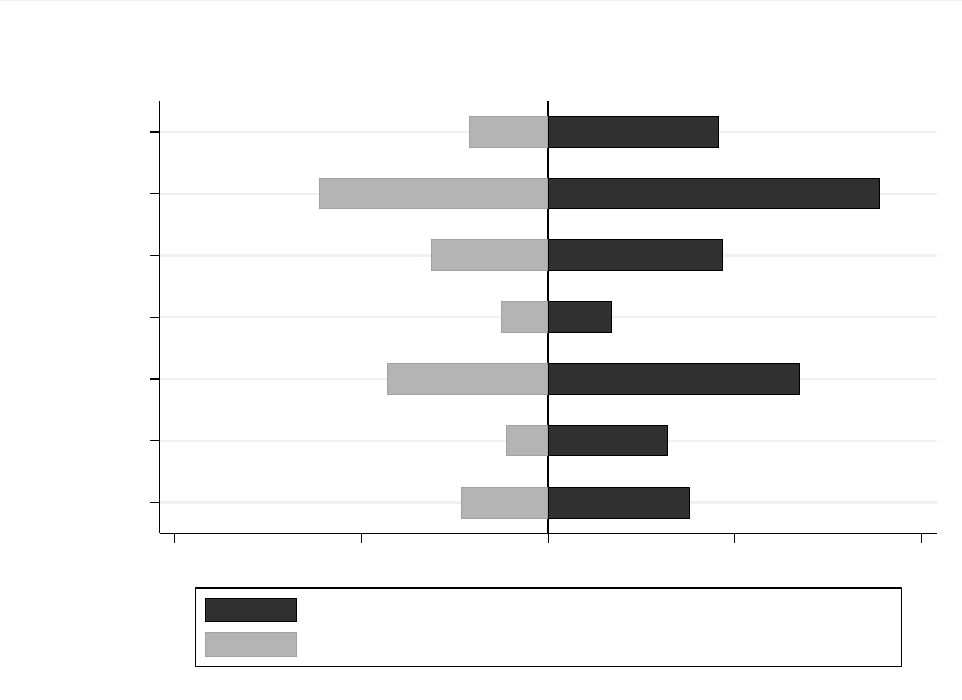
Figure 1
Notes: The bars show the share of jobs in each occupation category that required an “old” skill in 2007 (the light
gray bars) and a “new” skill in 2017 (the dark gray bars). Old skills are defined as those with at least 1,000
appearances in 2007 but a re ei ther fi ve ti mes l ess frequent or do not exi st i n 2017. New s ki ll s are defi ned as thos e
with at least 1,000 appearances in 2017 that either did not exist in 2007 or are 20 times more frequent in 2017
than 2007. The values of each bar are coefficients from a vacancy-level regression of the frequency of old and new
skill requirements on an indicator for the 2017 year, the total number of skills listed in each vacancy, education
and experience requirements, and occupation-city-empl oyer fi xed effects.
Management
STEM
Business
Social Service
Media/Design
Health
Sales/Admin
-.4 -.2 0 .2 .4
Share of job ads with new skill requirements in 2017
Share of job ads with old skill requirements in 2017
Professional Occupations
Turnover of Skill Requirements by Occupation Category
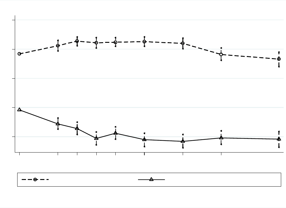
Figure 2
Notes: This figure shows how new skill requirements change along with required years of experience – i n STEM,
compared to other professional occupations. Each point in the figure is the coefficient (and associated 95 percent
confidence interval ) on the rel eva nt experi ence ca tegory from a vacancy-l evel regres si on of the frequency of new
skill requirements on experience categories, the total number of skills listed in the vacancy, education
requirements, and employer-by-MSA fi xed effects . New skills are defined as those with at least 1,000 appearances
in 2017 that either did not exist in 2007 or are 20 times more frequent in 2017 than 2007.
.2 .25 .3 .35 .4
0 to 1
2
3
4
5
6 to 7
8 to 9
10 to 11 12 or more
Years of Experience Required
STEM Occupations Other Professional Occupations
Regression includes controls for education requirements, the number of total skills, and employer fixed effects
Sample is 2017 BG Data, excluding vacancies with missing employer
New Skills Required by Job Experience
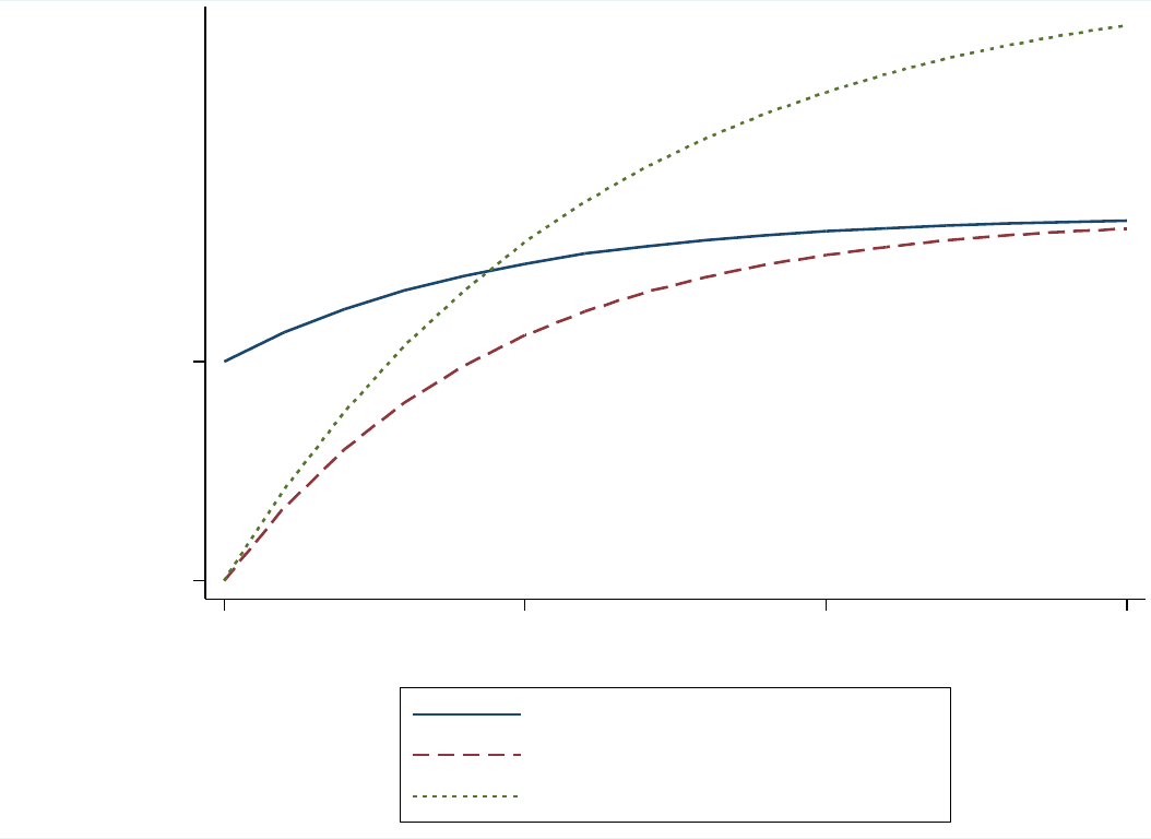
Figure 3A
Notes: This Figure simulates earnings growth from the model in Section 3 of the paper when
∗
= 6 (high in-school productivity) or
∗
= 3 (l ow
in-school productivity) and the rate of task change ∆
i s equal to 0.20 or 0.15. See the text for detai l s.
Impact of schooling diminishes over time
High delta = lower earnings growth
FjS*+a
(1/2)FjS* + a
Wages (Wjt)
0 5
10 15
Years since graduation
High in-school productivity; delta=0.2
Low in-school productivity; delta=0.2
Low in-school productivity; delta=0.15
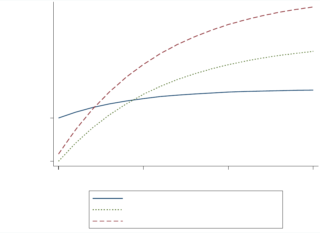
Figure 3B
Notes: This Figure simulates earnings growth from the model in Section 3 of the paper when
∗
= 6 (high in-school productivity) or
∗
= 3 (l ow
in-school productivity), the rate of task change ∆
is equal to 0.20 or 0.15, and for a high vs. low ability worker. See the text for deta i l s .
High ability workers learn more on the job, switch earlier into low delta fields
FjS*+a
(1/2)FjS*+a
Wages (Wjt)
0
5
10
15
Years since graduation
High in-school productivity; delta=0.2
Low in-school productivity, delta=0.15
Low in-school productivity, higher ability, delta=0.15
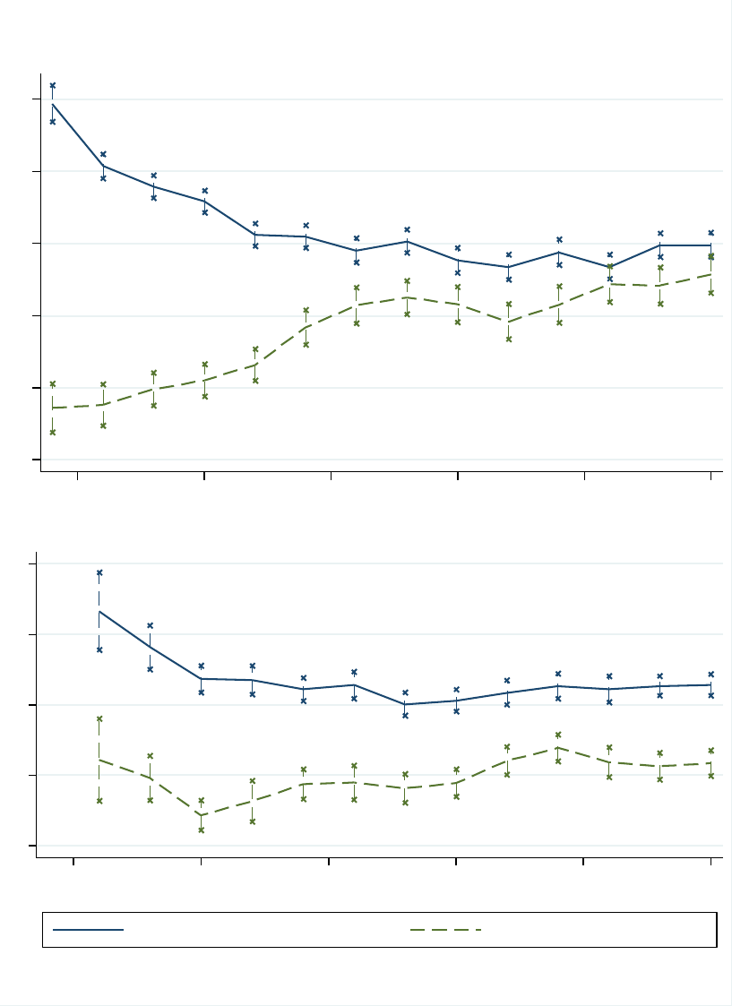
Figure 4
Notes: The figure plots coefficients and 95 percent confidence intervals from an estimate of the returns to majors
over time, following equation (10) in the paper. "Pure" Science includes biology, chemistry, physics, mathematics
and statistics, while "Applied" Science includes engineering and computer science.
-.1 0 .1 .2 .3 .4
25 30
35
40
45
50
Age (2 -year bins)
2009-2016 American Community Survey
0-.2 .2 .4 .6
25
30
35
40 45
50
Age (2 -year bins)
Applied Science Majors Pure Science Majors
Samples are full-time working men with a college degree; outcome is log wages
Left-out category is all other majors; includes demographic controls and age and year fixed effects
1993-2013 National Survey of College Graduates
Life-Cycle Returns to STEM Majors
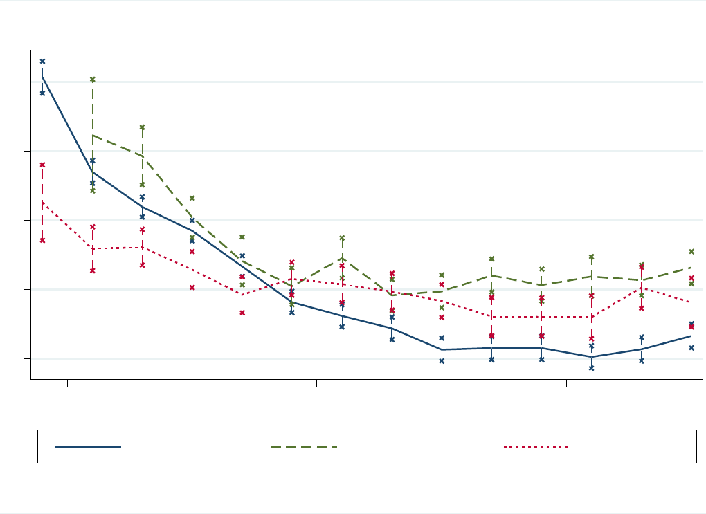
Figure 5
Notes: The figure plots coefficients and 95 percent confidence intervals from three separate es timates of equation (10) in the paper, except we
interact age bins with indicators for working in a STEM occupation rather than earning a STEM degree. STEM occupations are defined using the 2010
Census Bureau classification. The three data sources are the 2009-2016 American Community Survey, the 1993-2013 National Survey of College
Graduates, and the 1973-2016 Current Population Survey.
.1 .2 .3
.4 .5
25 30 35 40 45 50
Age (2 -year bins)
ACS NSCG
CPS
Sample is full-time working men with at least a college degree
Left-out category is all other majors; includes demographic controls and age and year fixed effects
Outcome is Log Wages
Life-Cycle Returns to Working in a STEM Occupation Across 3 Data Sources
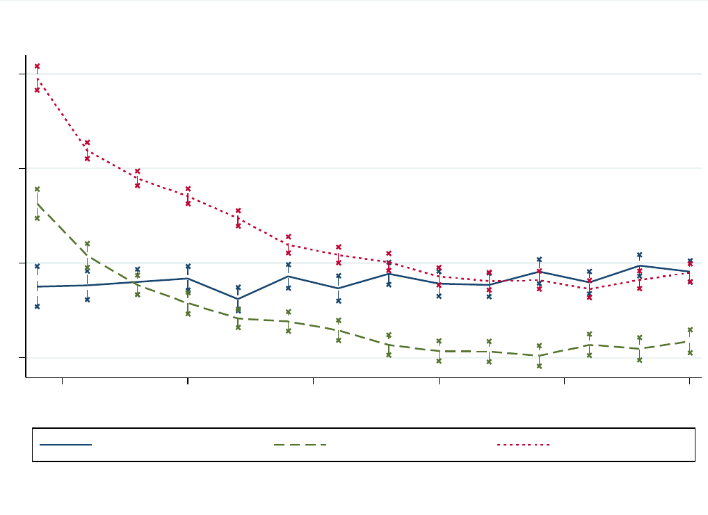
Figure 6
Notes: The fi gure plots coeffi ci ents and 95 percent confi dence i nterval s from an esti mate of the returns to maj ors over ti me, following equation (10) in
the paper, but adding occupation and major interactions. "Applied" Science majors include engineering and computer science.
0 .2
.4 .6
25 30 35 40
45 50
Age (2 -year bins)
Appl Sci, non-STEM job
Other Major, STEM Job
Appl Sci, STEM Job
Left-out category is other major, non-STEM job; includes demographic controls and age and year fixed effects
Sample is full-time working men with at least a college degree; 2009-2016 ACS
Outcome is Log Wages
Declining Returns for STEM Jobs, not STEM Majors
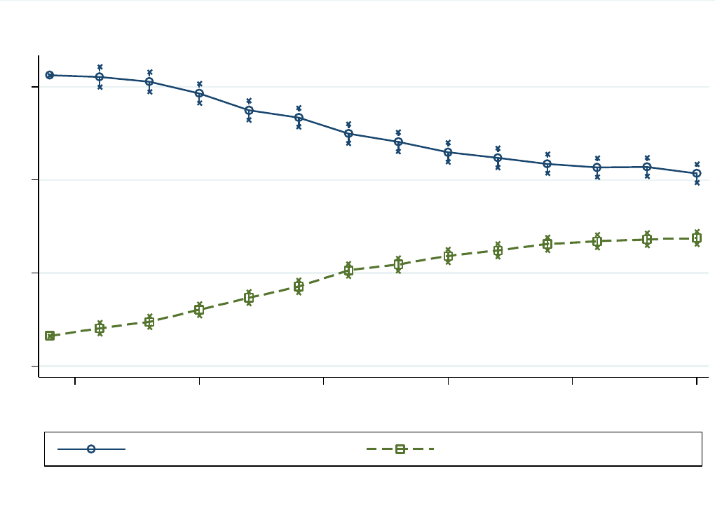
Figure 7
Notes: The figure plots coefficients and 95 percent confidence intervals from two separate es timates of equation (10) in the paper, restri cti ng the
sample to Applied Science majors and with indicators for working in STEM and management occupations as the outcome variables. STEM occupations
are defined using the 2010 Census Bureau classification.
0 .2 .4 .6
25 30 35
40 45 50
Age
STEM Occupations Management Occupations
Sample is full-time working men with at least a college degree; 2009-2016 ACS
Includes demographic controls and age and year fixed effects
Outcome is the share working in each occupation category
Occupational Sorting over Time for Applied Science Majors
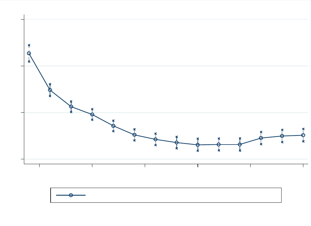
Figure 8
Notes: The figure plots coefficients and 95 percent confidence intervals from an estimate of equation (11) in the paper, a regression of log wages on
i nteracti ons between two-year age bins and the skill change measure ∆
that i s estimated using 2007-2017 online job vacancy data from Burning Glass
Technol ogi es . The standard deviation of ∆
is 1.14, indicating that jobs with a 1 SD higher skill change pay 24 percent higher wages at ages 23-24 but
only 13 percent higher at ages 49-50. STEM occupations are defined using the 2010 Census Bureau classification. See the text for details.
.1
.15 .2 .25
Log Wages
25
30 35 40
45 50
Age (2 year bins)
Wage return to a 1 SD increase in job skill change
Sample is full-time working men with at least a college degree; 2009-2016 ACS
Includes demographic controls and age and year fixed effects
Jobs with Higher Rates of Skill Change Pay More to Younger Workers

Figure 9
Notes: The figure plots coefficients and 95 percent confidence intervals from an estimate of equation (12) in the paper, a regression of the task change
meas ure ∆
(which is constructed using 2007-2017 online job vacancy data from Burning Glass Technologies) on occupation by age group interactions.
The standard deviation of ∆
is 1.14, indicating that workers age 23-24 are in jobs that score about 0.2 standard deviations higher on the job skill
change mea sure than workers age 49-50. STEM occupations are defined using the 2010 Census Bureau classification. See the text for details.
-.05 0
.05 .1 .15
.2
Job Skill Change
25
30 35 40
45
50
Age (2 year bins)
Sample: Full-time working men with at least a college degree; 2009-2016 ACS
Left-out category is age 49-50; includes demographic controls and age and year fixed effects
Younger Workers in Jobs with Higher Rates of Skill Change
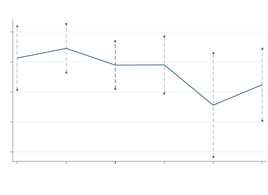
Figure 10
Notes: The figure plots coefficients and 95 percent confidence intervals from an estimate of equation (10) in the paper, which regresses log wages on
major-by-age group interactions. "Applied" Science includes engineering and computer sci ence ma jors. The regres si on is esti mated at the person-year
level and standard errors are cl us tered a t the i ndivi dual l evel . The s a mple i s restri cted to ages 23-34 to ensure compa rabil ity across NLSY wa ves.
-.1 0 .1 .2 .3
24
26
28
30 32
34
Age (2 -year bins)
Sample is full-time working men with at least a college degree; NLSY79 and NLSY97 (Pooled)
Includes demographic controls, age and year fixed effects, AFQT and noncognitive skills
Outcome is Log Wages
Declining Life-Cycle Returns to Applied Science Majors
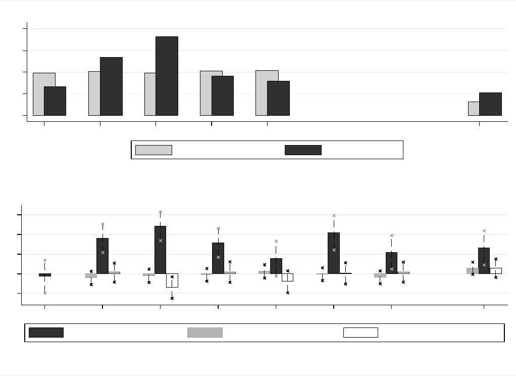
Figure 11
Notes: Pa nel A pres ents es ti mates of the task cha nge measure ∆
calculated using data from Atalay et al (2018) on the text of classified job ads
between the years of 1977 and 1999. Panel B presents coefficients and 95 percent confidence intervals from a regression of log wages on age (23-26
vs. 27-50) by STEM occupation interactions for successive five year periods that match the job ad data, using the CPS. STEM occupations are defined
using the 2010 Census Bureau classification. See the text for details.
Task data from text of classified ads, as in Atalay et al (2018)
Task data from online job vacancies, 2007-2017
0 .2 .4 .6 .8
1978 1983 1988
1993
1998 2017
Non-STEM Occupations STEM Occupations
Calculated over five year periods beginning with 1973-1978; see text for details
1973-1998 data taken from Atalay et al (2018); 2007-2017 data from Burning Glass
Rate of Within-Occupation Task Change, by Period
-.1 0 .1 .2 .3
1978 1983
1988 1993 1998
2003 2008
2016
Young STEM workers Older STEM workers Young non-STEM workers
Sample is full-time men with at least a college degree; 1973-2016 CPS
Outcome is log wages; includes controls for demographics and age and year fixed effects; "young" is age 23-26
Young STEM Workers Earn More During Periods of Rapid Task Change

Table 1: Skill Requirements by Occupation Category in 2007
Panel A Social C
ognitive Character Creativity Writing Management Finance
(1) (2) (3) (4) (5) (6) (7)
Management 0.606 0.421 0.453 0.077 0.172 0.382 0.402
STEM 0.540 0.536 0.345 0.063 0.208 0.170 0.167
Business 0.651 0.551 0.463 0.100 0.182 0.258 0.475
Social Science / Service 0.362 0.356 0.220 0.062 0.158 0.147 0.081
Art/Design/Media 0.585 0.397 0.502 0.256 0.465 0.138 0.160
Health 0.331 0.238 0.190 0.021 0.063 0.136 0.053
Sales and Admin 0.626 0.321 0.423 0.073 0.127 0.180 0.222
Total 0.566 0.458 0.386 0.077 0.177 0.213 0.269
Panel B
Business
Systems
Customer
Service
Office
Software
Technical
Support
Data
Analysis
Specialized
Software
ML and AI
Management 0.243 0.315 0.
296 0.115 0.057 0.209 0.005
STEM 0.260 0.207 0.254 0.328 0.092 0.593 0.039
Business 0.272 0.340 0.394 0.123 0.083 0.260 0.006
Social Science / Service 0.045 0.134 0.151 0.053 0.023 0.094 0.003
Art/Design/Media 0.125 0.195 0.337 0.153 0.029 0.396 0.009
Health 0.022 0.392 0.139 0.037 0.026 0.048 0.002
Sales and Admin 0.193 0.763 0.331 0.126 0.040 0.156 0.011
Total 0.218 0.354 0.296 0.177 0.067 0.320 0.017
Notes: Each cell in this table presents the share of postings in an occupation category that requires at least one skill in
the categories indicated in each column. The occupations are grouped based on 2010 Standard Occupation Classification
(
SOC) codes. Data come from online job vacancies collected by Burning Glass Technologies in 2007. See the Data Appendix
for detailed descriptions of how each skill category is constructed.

Table 2: Skill Requirements by Occupation Category in 2017
Panel A Social Cognitive Character Creativity Writing Management Finance
(1) (2) (3) (4) (5) (6) (7)
Management 0.715 0.515 0.552 0.117 0.221 0.447 0.461
STEM 0.659 0.644 0.448 0.112 0.252 0.208 0.189
Business 0.766 0.642 0.606 0.147 0.243 0.299 0.487
Social Science / Service 0.516 0.382 0.336 0.096 0.197 0.184 0.080
Art/Design/Media 0.700 0.476 0.610 0.365 0.497 0.162 0.189
Health 0.438 0.299 0.284 0.032 0.070 0.163 0.051
Sales and Admin 0.758 0.444 0.613 0.098 0.173 0.235 0.312
Total 0.661 0.531 0.489 0.114 0.214 0.253 0.278
Panel B
Business
Systems
Customer
Service
Office
Software
Technical
Support
Data
Analysis
Specialized
Software
ML and AI
Management 0.292 0.363 0.370 0.094 0.084 0.253 0.021
STEM 0.304 0.220 0.284 0.329 0.170 0.679 0.180
Business 0.362 0.397 0.488 0.092 0.119 0.351 0.029
Social Science / Service 0.043 0.157 0.190 0.040 0.049 0.110 0.015
Art/Design/Media 0.136 0.195 0.372 0.105 0.055 0.472 0.024
Health 0.031 0.558 0.154 0.028 0.040 0.099 0.005
Sales and Admin 0.274 0.760 0.429 0.076 0.058 0.237 0.016
Total 0.249 0.381 0.335 0.145 0.104 0.367 0.065
Notes: Each cell in this table presents the share of postings in an occupation category that requires at least one skill in
the categories indicated in each column. The occupations are grouped based on 2010 Standard Occupation Classification
(SOC) codes. Data come from online job vacancies collected by Burning Glass Technologies in 2017. See the Data Appendix
for detailed descriptions of how each skill category is constructed.

SOC code Occupation Title
Rate of Task
Change
SOC code Occupation Title
Rate of Task
Change
172 Engineers 3.53 151131 Computer Programmers 6.69
192 Physical Scientists 3.48 151133 Software Developers, Systems Software 5.99
191 Life Scientists 3.25 172081 Environmental Engineers 5.49
151 Computer Occupations 3.24 151142 Network / Computer Systems Administrators 4.71
113 Operations Specialties Managers 3.20 173013 Mechanical Drafters 4.49
152 Mathematical Scientists 3.19 172041 Chemical Engineers 4.37
171 Architects and Surveyors 3.13 152041 Statisticians 4.29
112 Advertising, Marketing and Sales Managers 3.00 151141 Database Administrators 3.98
132 Financial Specialists 2.71 151134 Web Developers 3.96
173 Drafters and Engineering Technicians 2.61 151152 Computer Network Support Specialists 3.77
SOC code Occupation Title
Rate of Task
Change
SOC code Occupation Title
Rate of Task
Change
252 Pre-K, Primary and Secondary School Teachers 0.74 291021 Dentists 0.32
253 Other Teachers and Instructors 0.79 291066 Psychiatrists 0.38
291 Health Diagnosing and Treating Practitioners 0.86 193031 Clinical Psychologists 0.41
272 Entertainers and Performers 1.12 291069 Physicians and Surgeons, All Other 0.41
259 Other Education, Training and Library Occupations 1.15 291062 Family and General Practitioners 0.41
292 Health Technologists and Technicians 1.29 291171 Nurse Practitioners 0.44
251 Postsecondary Teachers 1.36 252059 Special Education Teachers, All Other 0.46
193 Social Scientists and Related Workers 1.40 252031 Secondary School Teachers 0.51
211 Counselors and Social Workers 1.51 292052 Pharmacy Technicians 0.54
274 Media / Communications Equipment Workers 1.76 272022 Coaches and Scouts 0.63
Notes: This table uses online job vacancy data from Burning Glass Technologies (BG) to calculate the rate of skill change between 2007 and 2017 for each 3- and 6-digit
Standard Occupational Classification (SOC) code. The average value of the task change measure is 2.10 - see the text for details. Professional Occupations are SOC codes that
begin with a 1 or a 2.
Table 3: Occupations with the Highest and Lowest Rates of Task Change
Panel A: Fastest-Changing Professional Occupations (3-digit)
Panel B: Fastest-Changing Professional Occupations (6-digit)
Panel C: Slowest-Changing Professional Occupations (3-digit)
Panel D: Slowest-Changing Professional Occupations (6-digit)

Age Wages
Share in
STEM Job
Wages
Share in
STEM Job
Wages
Share in
STEM Job
(1) (2) (3) (4) (5) (6)
23 32,236 0.074 32,840 0.269 47,007 0.616
24 36,632 0.076 35,909 0.286 52,727 0.631
25 43,354 0.076 44,849 0.258 58,188 0.620
26 46,918 0.075 49,472 0.282 61,558 0.616
27 51,722 0.075 53,181 0.247 66,286 0.626
28 54,856 0.074 57,243 0.231 69,590 0.585
29 58,389 0.073 62,651 0.238 73,765 0.584
30 62,787 0.074 69,109 0.224 76,309 0.569
31 67,567 0.074 79,274 0.220 80,546 0.539
32 71,933 0.074 79,894 0.212 83,536 0.536
33 74,608 0.072 91,085 0.211 89,109 0.525
34 79,971 0.069 98,442 0.206 91,542 0.515
35 85,897 0.069 105,914 0.205 98,291 0.482
36 89,875 0.070 111,807 0.198 99,114 0.487
37 93,259 0.073 114,927 0.206 103,804 0.472
38 94,453 0.072 117,943 0.194 108,081 0.463
39 99,481 0.065 121,372 0.189 110,477 0.461
40 99,952 0.069 123,224 0.199 111,678 0.429
41 103,447 0.066 123,281 0.187 113,388 0.425
42 104,068 0.067 122,578 0.199 113,511 0.439
43 106,122 0.068 132,626 0.194 120,005 0.422
44 108,777 0.064 129,115 0.194 122,278 0.419
45 111,802 0.061 136,001 0.204 121,420 0.427
46 111,235 0.062 141,341 0.179 121,746 0.399
47 112,430 0.060 136,539 0.199 125,350 0.418
48 112,002 0.058 136,772 0.206 126,601 0.410
49 112,347 0.059 139,118 0.204 126,111 0.403
50 111,754 0.060 137,439 0.204 126,606 0.399
Notes: This table presents population-weighted average annual wage and salary income and
employment shares in Science, Technology, Engineering and Mathematics (STEM) occupations by
age, using the 2009-2016 American Community Survey Integrated Public Use Microdata Series
(IPUMS, Ruggl es et al 2017). The sampl e i s restri cted to men wi th at l ea s t a col lege degree who
were empl oyed a t the ti me of the survey and worked at l eas t 40 weeks during the year. Earni ngs
are in constant 2016 dollars. STEM majors are defined following Peri, Shih and Sparber (2015),
and STEM jobs are defined using the 2010 Census Bureau classification. "Pure" Science includes
biology, chemistry, physics, mathematics and statistics, while "Applied" Science includes
engineering and computer science.
Table 4: Life-Cycle Earnings and Employment for STEM Majors
Non-STEM Major
"Pure" Science
"Applied" Science

Table 5: Labor Market Returns to STEM Majors in the NLSY
Outcome is Log Hourly Wage (2016$) (1) (2) (3) (4) (5) (6)
Applied Science Major 0.179*** 0.180*** 0.072* 0.034 0.013 0.046
[0.035] [0.036] [0.037] [0.034] [0.041] [0.044]
Pure Science Major -0.099 -0.103 -0.141* -0.107* -0.110 -0.037
[0.079] [0.074] [0.073] [0.058] [0.067] [0.063]
STEM Occupation 0.241*** 0.143*** 0.119***
[0.028] [0.027] [0.029]
Applied Science * STEM Occupation 0.057
[0.051]
Pure Science * STEM Occupation 0.031
[0.112]
Cognitive Skills (AFQT, standardized) 0.129*** 0.113*** 0.076*** 0.076*** 0.063
[0.025] [0.024] [0.021] [0.021] [0.031]
Social Skills (standardized) 0.042*** 0.048*** 0.033*** 0.033*** 0.009
[0.015] [0.014] [0.012] [0.012] [0.015]
Noncognitive Skills (standardized) 0.060*** 0.058*** 0.045*** 0.045*** 0.041
[0.016] [0.016] [0.013] [0.013] [0.016]
Demographics and Age/Year FE X X X X X X
Industry Fixed Effects X X
Occupation-by-Industry Fixed Effects X
R-squared 0.225 0.244 0.259 0.397 0.397 0.649
Number of Observations 8,634 8,634 8,634 8,634 8,634 8,634
Notes: Each column reports results from a regression of real log hourly wages on indicators for college major,
occupation and/or industry (in columns 3 through 5), individual skills, indicator variables for race and years of
completed education, age and year fixed effects, and additional controls as indicated. The data source is the
National Longitudinal Survey of Youth (NLSY) 1979 and 1997, and the sample is restricted to men with at least a
college degree. The waves are pooled and an indicator for sample wave is included in the regression. Science,
Technology, Engineering and Mathematics (STEM) occupations are defined using the 2010 Census Bureau
classification. "Pure" Science majors include biology, chemistry, physics, mathematics and statistics, while
"Applied" Science includes engineering and computer science. Cognitive skills are measured by each respondent's
score on the Armed Forces Quali fying Tes t (AFQT). We norma l i ze scores a cross NLSY wa ves usi ng the crosswal k
developed by Altonji, Bharadwaj and Lange (2012). Social and noncognitive skill definitions are taken from Deming
(2017). All skill measures are normalized to have a mean of zero and a standard deviation of one. Person-year is the
unit of observation, and all standard errors are clustered at the person level. The sample is restricted to ages 23-34
to maxi mi ze comparabil i ty acros s survey wa ves. *** p<0.01, ** p<0.05, * p<0.10.

Table 6: STEM Majors, Relative Wages and Ability Sorting in the NLSY
In a STEM Job
(
1) (2) (3)
STEM Major 0.352*** 0.116*** 0.005
[0.035] [0.034] [0.120]
AFQT (Standardized) 0.084*** 0.063* 0.017
[0.016] [0.033] [0.032]
Age (Linear) 0.002 0.013 0.007
[0.005] [0.008] [0.009]
Age * AFQT -0.005** 0.013*** 0.024***
[0.002] [0.005] [0.005]
Age * STEM Major 0.027*
[0.014]
STEM Major * AFQT 0.187*
[0.097]
STEM Major * AFQT * Age -0.041***
[0.013]
R-squared 0.183 0.237 0.242
Number of Observations 11,214 8,685 8,685
Notes: Each column reports results from a regression of indicators for working
in a STEM occupation (Column 1) or real log hourly wages (Columns 2 and 3)
on indicators for majoring in a Science, Technology, Engineering and
Mathematics (STEM) field, cognitive, social and noncognitive skills, indicator
variables for race and years of completed education, year fixed effects, and
additional controls as indicated. The data source is the National Longitudinal
Survey of Youth (NLSY) 1979 and 1997, and the sample is restricted to men with
at l east a col l ege degree. The waves are pool ed and an i ndi ca tor for sampl e
wave is included in the regression. STEM majors are defined following Peri,
Shih and Sparber (2015), and STEM occupations are defined using the 2010
Census Bureau classification. Cognitive skills are measured by each
respondent's score on the Armed Forces Qualifying Test (AFQT). We normalize
scores across NLSY waves using the crosswalk developed by Altonji,
Bharadwaj and Lange (2012). Social and noncognitive skill definitions are
taken from Demi ng (2017). Al l s kil l measures are normal i zed to have a mean of
zero and a standard deviation of one. Person-year is the unit of observation,
and all standard errors are clustered at the person level. The sample is
res tri cted to ages 23-34 to maximi ze comparabi l i ty a cros s s urvey waves . ***
p<0.01, ** p<0.05, * p<0.10.
Ln (Wages)
