1 of 24
September 2008 Dr. Robert Gebotys
Example: Quadratic Linear Model
Gebotys and Roberts (1989) were interested in examining
the effects of one variable (i.e. “age’) on the “seriousness
rating of the crime” (y); however, they wanted to fit a
quadratic curve to the data. The variables to be examined
within this example are “age” and “age squared” (i.e.,
‘agesq’). The model is: E(y|x)= B
0
+ B
1
age + B
2
age
2
Complete the following steps in the Linear regression
utilizing SPSS in order to follow the output explanation
starting on page thirteen.
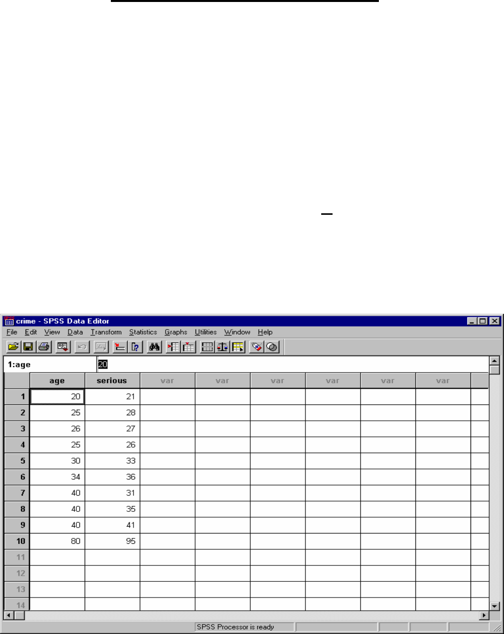
1. Pull up “Crime” data set. (or enter data below)

2 of 24
September 2008 Dr. Robert Gebotys
Before proceeding to any analysis, the new variable
‘agesq’ needs to be created. To create ‘agesq’ do the
following:
1. Click Transform on the main menu bar.
2. Click Compute on the Transform menu. You
should now see the following box:

3 of 24
September 2008 Dr. Robert Gebotys
3. Type ‘agesq’ in the Target Variable text box,
located at the top left corner of the Compute
Variable dialogue box. This is to specify the new
variable that you are creating, ‘agesq’.
4. To specify the numeric expression of ‘agesq’ (that
is, the squaring of ‘age’), click “age” in the variable
source list and click the arrow button to the right
of the variable source list box. Then click the “**”
button on the lower right-hand side of the on-
screen key pad followed by clicking the ‘2’ button
on the keypad. As a result of the above clicks, the
expression “age**2”will be entered into the
Numeric Expression box.
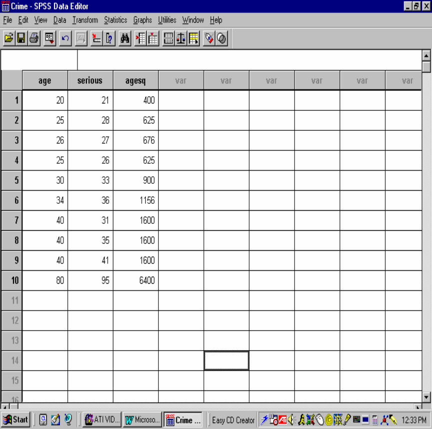
5. Click the ‘OK’ command pushbutton of the
dialogue box. You will immediately see that a new
variable, ‘agesq’, has been entered into the Data
Editor. (Note
that the variable ‘agesq’ is set to two
decimal points. If you would like to re-set this
variable to “zero” decimal points to be congruent
4 of 24
September 2008 Dr. Robert Gebotys
with other variables do the following: (i) Double
click on ‘agesq’ variable label to “Define label
box”; (ii) See section called ‘Change settings’ and
click Type button; (iii) Change decimal places from
“2” to “0”; (iv) Click button Continue; and finally
(v) Click the ‘OK’ button. Your ‘agesq’ variable
should now contain no decimal places).

5 of 24
September 2008 Dr. Robert Gebotys
6. At this stage, you may save the data matrix on a
diskette, for example, under the file name
“crimeage2.sav”.
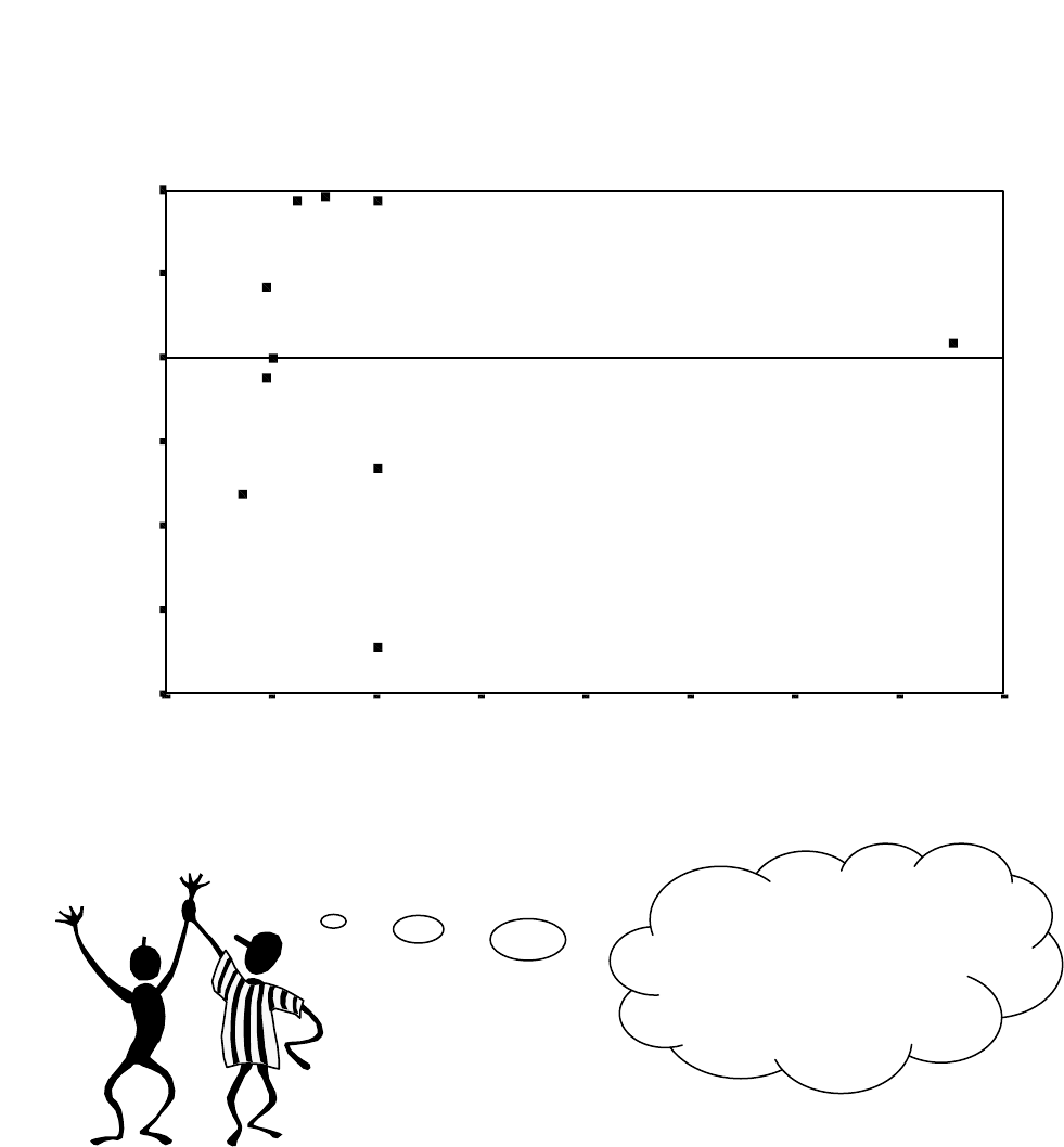
Fitting a Quadratic Regression Curve on the Scatterplot
1. Start by creating a scatterplot for the set of data on
age and crime seriousness.
2. To fit a quadratic regression curve, start by
clicking on the scatterplot as it appears in the
Results pane of the SPSS viewer window so that a
thin black line surrounds the scatterplot. Next,
click on Edit on the menu bar and select SPSS
Chart Object from the E
dit menu, followed by
clicking O
pen on the submenu. This series of clicks
will open a SPSS Chart Editor window. The
scatterplot you have produced will appear in the
Chart Editor window.
6 of 24
September 2008 Dr. Robert Gebotys
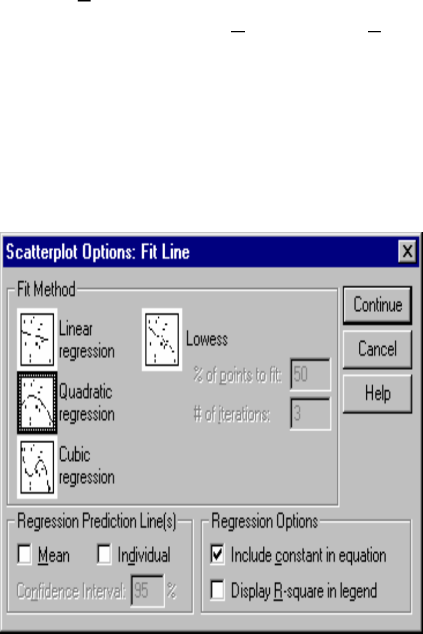
3. Click Chart on the Chart Editor window menu
bar, followed by clicking ‘O
ptions…’ in the Chart
menu. When the ‘Scatterplot Options’ dialogue
box is activated, click the check box to the left of
the Total in the ‘Fit Line’ box. Then click the ‘Fit
Options…’ button in the ‘Fit Line’ box. This will
open a ‘Scatterplot Options: Fit Line’ dialogue box
as shown below.
7 of 24
September 2008 Dr. Robert Gebotys
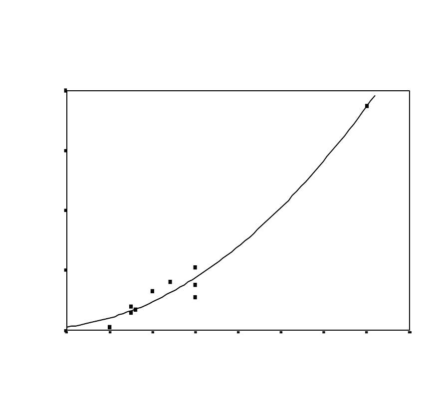
4. Click the ‘Quadratic regression’ box. Click the
‘Continue’ pushbutton. When the ‘Scatterplot
Options’ dialogue box reappears, click the ‘OK’
command pushbutton. After a few seconds, you
should see that a curve has already been fit to the
scatterplot. A copy of the scatterplot is reproduced
below. At this stage you can edit, save, and print
the scatterplot.
Scatterplot of "Serious" vs "Age"
Quadratic Line Fit
AGE
908070605040302010
SERIOUS
100
80
60
40
20
8 of 24
September 2008 Dr. Robert Gebotys
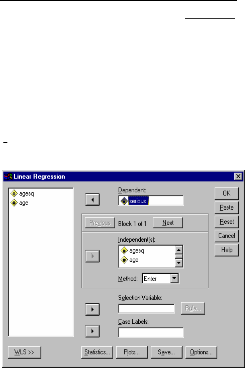
Specifying the Regression Procedure for a Polynomial
of Degree 2
Follow the Regression Procedure in “Example: The
Linear Model with Normal Error”. The one exception
is that both ‘age’ and ‘agesq’ should be defined as the
independent variables in this model. This is done by
clicking both ‘age’ and ‘agesq’ in the variable source
list and then clicking the arrow button to the left of the
‘I
ndependent[s:’ text box. The dialogue box should now
resemble the one below.

9 of 24
September 2008 Dr. Robert Gebotys
After completing the procedures as specified in the
“Example: Linear Model with Normal Error” (i.e.
designate ‘Statistics’, ‘Plots’ and ‘Save’ selections for
this analysis), then click the ‘OK’ command pushbutton
in the Linear Regression dialogue box. This will
instruct SPSS to produce a set of output similar to that
to be discussed in the next section.
Alternate Method to Perform Linear Regression
This is performed by utilizing the Run command in a SPSS
Syntax window. That is, the selections you have made in the
Linear Regression dialogue boxes are actually commands
for the regression procedure. You can click the Paste
command pushbutton in the Linear Regression dialogue
box to paste this underlying command syntax into a Syntax
window (i.e., a syntax window will be opened when the
Paste command is clicked and the selections that you have
made are reproduced in this window in the format of a
command syntax or SPSS programming language).

10 of 24
September 2008 Dr. Robert Gebotys
There is another way of specifying and running the
regression procedure for fitting the quadratic model. If
you have already saved the syntax commands in a file
(e.g., crime.sps), as outlined in “Example: Linear Model
with Normal Error”, you can specify and run the
regression procedure by following the steps described
below:
1. Insert the diskette containing the relevant file (e.g.,
crime.sps) into drive A.
2. Click F
ile on the main menu bar.
3. Click Open in the File menu to activate and open
File dialogue box.
4. Check if the current position of the drive (i.e. the
“Look in” text box) is drive A. If not, change it to
drive A by clicking on the arrow to the right of the
text box and selecting “3.5 Floppy [A:]”.

11 of 24
September 2008 Dr. Robert Gebotys
5. Check if the File type text box contains “SPSS
syntax files (*.sps)”. If not, change it by clicking on
the arrow to the right of the text box and selecting
that option using a single click.
6. The relevant file (e.g., crime.sps) should now be
listed in the large text box in the centre of the Open
File dialogue box. Select the file with a single click
and then proceed to that file by clicking the Open
command pushbutton. This will open a window
titled “crime – SPSS Syntax Editor”.
Sometimes the only ‘problem’
is the solution to the
‘problem’…….That’s it!
Focus on entering the syntax
correctly……..then there is
no ‘problem’, only ‘solutions’
or in SPSS lingo, ‘output’.
12 of 24
September 2008 Dr. Robert Gebotys
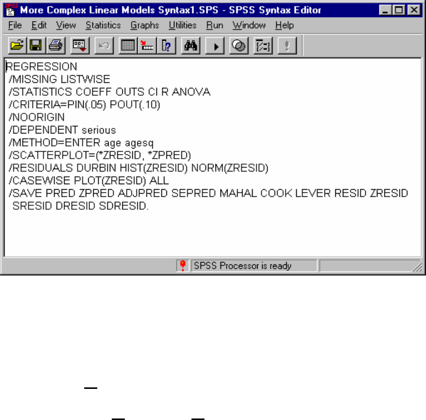
7. Go to the end of the line “/METHOD=ENTER
age” and click once to move your cursor/pointer to
that location. Add a space after ‘age’ and then
type ‘agesq’. Your command syntax should now
look like that listed below:
If you want to save or print this syntax window,
you may do so now.
8. Click ‘R
un’ on the Syntax Editor menu bar, and
then click A
ll on the Run menu. This will instruct
the computer to perform the required regression
procedure.

13 of 24
September 2008 Dr. Robert Gebotys
Quadratic Linear Model
SPSS Output Explanation
The REGRESSION command fits linear models by
least squares. The METHOD subcommand tells SPSS
what variables are in the model. The DEPENDENT
subcommand tells SPSS which is the y variable. The
ENTER command defines the x variables. In this case
we have asked SPSS to fit the model.
E(y|x)=B
0
+ B
1
x + B
2
x
2
The output, using SPSS windows or syntax, is
interpreted as follows:
Variables Entered/Removed
b
AGESQ,
AGE
a
. Enter
Model
1
Variables
Entered
Variables
Removed
Method
All requested variables entered.
a.
Dependent Variable: SERIOUS
b.

14 of 24
September 2008 Dr. Robert Gebotys
ANOVA
b
3896.297 2 1948.149 139.434 .000
a
97.803 7 13.972
3994.100 9
Regression
Residual
Total
Model
1
Sum of
Squares
df
Mean
Square
F Sig.
Predictors: (Constant), AGESQ, AGE
a.
Dependent Variable: SERIOUS
b.
Model Summary
b
.988
a
.976 .969 3.74 2.081
Model
1
R R Square
Adjusted R
Square
Std. Error
of the
Estimate
Durbin-Watson
Predictors: (Constant), AGESQ, AGE
a.
Dependent Variable: SERIOUS
b.
Coefficients
a
20.683 8.823 2.344 .052 -.180 41.545
-8.49E-02 .410 -.069 -.207 .842 -1.055 .885
1.262E-02 .004 1.055 3.174 .016 .003 .022
(Constant)
AGE
AGESQ
Model
1
B Std. Error
Unstandardized
Coefficients
Beta
Standardi
zed
Coefficien
ts
t Sig.
Lower
Bound
Upper
Bound
95% Confidence Interval
for B
Dependent Variable: SERIOUS
a.
15 of 24
September 2008 Dr. Robert Gebotys
In order to determine if the model is adequate we
examine the ANOVA table. Note the degrees of
freedom and F-statistic values.
F = 139.434
which has an F distribution with 2
(number of
parameters [3] – intercept B
0
[1] = 3 – 1 = 2) and 7
(number of observations – number of parameters
= 10 – 3 = 7) degrees of freedom. We reject
H
o
: B
1
= B
2
= 0
H
a
: B
1
≠
B
2
≠
0
with p-value less than .0001, the SIGNIF value on the
output. The REGRESSION row refers to the model
and the RESIDUAL row refers to the error component.
The mean square of the residual is equal to s
2
,
our
estimate of sigma
2
, note s is also printed in the STD
ERROR OF THE ESTIMATE column.
s
2
= MSE= 13.972
s= 3.74
16 of 24
September 2008 Dr. Robert Gebotys
In the same area we also have R
2
, R SQUARE printed
where:
R
2
=
SSM/SST
= 3896/3994
= .97551
In other words 97.551% of the variance in seriousness is
accounted for by the model (‘age’, ‘agesq’).
In the Coefficients section the column model
variable lists the variable ‘age’, ‘agesq’ and ‘constant’
these refer to the variables associated with the
parameters B
0
, B
1
, and B
2
in the model. The column
labeled B given the least squares (b
0
= 20.683,
B
1
= -.085, b
2
= .0126) estimator for B
0
, B
1
, and B
2
.
The equation is therefore
E(y|x) = 20.683 – 085x + .012x
2
.
17 of 24
September 2008 Dr. Robert Gebotys
The STD ERROR column is the standard error column for
each of the parameters for example
s(b
0
) = 8.823
s(b
1
) = .410
s(b
2
) = .004
the T column gives the corresponding t statistic for testing
the hypothesis
H
0
: B
1
= 0
H
a
: B
1
≠
0
T = b
1
/s(b
1
) = -.207
H
0
: B
2
= 0
H
a
: B
2
≠
0
T = 3.174
For B
1
the t statistic has the value -.207, and for B
2
the t statistic has the value 3.174. The column SIG gives
the OLS or p-value for the test above. In this case we have
p=.842 for B
1
(not significant, therefore we cannot reject
H
0
) and p=.016 for B
2
(significant, therefore we can reject
H
0
); however, p=.016 for B
2
, therefore there is strong
evidence against H
0
. Both are with 7 degrees of freedom.

18 of 24
September 2008 Dr. Robert Gebotys
Casewise diagnostics gives a STD RESIDUAL COL with
STANDARDIZED VALUES between
≠
3. standard
deviations which is reasonable. The Du
rbin-Watson
Statistic is about 2 which indicates zero correlation. The
leverage (LEVER) and Cook’s distance (COOK D) values
for the 10
th
observation are relatively large
(h
10
= .8977, D = 405.069) indicating this is an influential
observation. If we compare h
10
to 2meanh where
meanh = .2 (found in the summary statistics section) our
suspicion that the 10
th
observation (a person 80 year old
with a high seriousness rating) is influential is confirmed.
Notice that the residual for this observation is small and
therefore not an outlier.
Casewise Diagnostics
a
-.812 21 24.04 -3.04
.414 28 26.45 1.55
-.003 27 27.01 -1.08E-02
-.121 26 26.45 -.45
.937 33 29.50 3.50
.965 36 32.39 3.61
-1.736 31 37.49 -6.49
-.666 35 37.49 -2.49
.939 41 37.49 3.51
.082 95 94.69 .31
Case Number
1
2
3
4
5
6
7
8
9
10
Std.
Residual
SERIOUS
Predicted
Value
Residual
Dependent Variable: SERIOUS
a.

19 of 24
September 2008 Dr. Robert Gebotys
Residuals Statistics
a
24.04 94.69 37.30 20.81 10
-.638 2.758 .000 1.000 10
1.28 3.73 1.93 .72 10
-35.46 39.73 24.58 21.72 10
-6.49 3.61 -7.11E-16 3.30 10
-1.736 .965 .000 .882 10
-2.013 1.690 .127 1.156 10
-8.73 130.46 12.72 41.60 10
-2.872 2.034 .077 1.400 10
.148 8.079 1.800 2.357 10
.000 405.070 40.618 128.055 10
.016 .898 .200 .262 10
Predicted Value
Std. Predicted Value
Standard Error of
Predicted Value
Adjusted Predicted Value
Residual
Std. Residual
Stud. Residual
Deleted Residual
Stud. Deleted Residual
Mahal. Distance
Cook's Distance
Centered Leverage Value
Minimum Maximum Mean
Std.
Deviation
N
Dependent Variable: SERIOUS
a.
Look we got
studentized and
other residual
statistics without
asking for them.
Bonus!
20 of 24
September 2008 Dr. Robert Gebotys
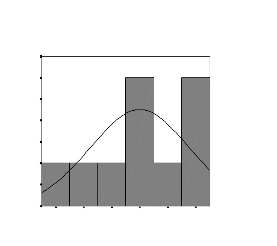
The histogram of residuals looks reasonable, although
with 10 observations, this is difficult to judge.
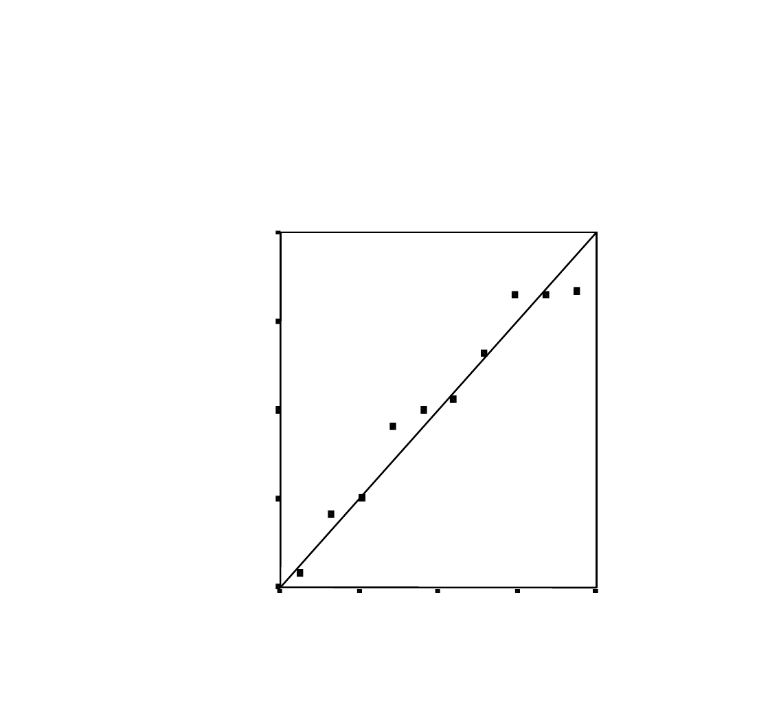
The probability plot has improved, from the previous
“Example: Linear Model with Normal Error”, in the
sense that the residuals more closely approximate a
normal distribution. The large bulge present in the
Regression Standardized Residual
1.00.500.00-.50-1.00-1.50
Histogram
Dependent Variable: SERIOUS
Frequency
3.5
3.0
2.5
2.0
1.5
1.0
.5
0.0
Std. Dev = .88
Mean = 0.00
N = 10.00
21 of 24
September 2008 Dr. Robert Gebotys
normal probability plot of residuals in the “Example:
Linear Model with Normal Error” is no longer present
in the polynomial of degree 2 model.
Normal P-P Plot of Regression
Standardized Residual
Dependent Variable: SERIOUS
Observed Cum Prob
1.00.75.50.250.00
Ex
pe
cte
d
Cu
m
Pr
ob
1.00
.75
.50
.25
0.00
22 of 24
September 2008 Dr. Robert Gebotys
The plot of y predicted vs e, displays a reasonable band
shape as
well.
Scatterplot
Dependent Variable: SERIOUS
Regression Standardized Predicted Value
3.02.52.01.51.0.50.0-.5-1.0
Regression Standardized Residual
1.0
.5
0.0
-.5
-1.0
-1.5
-2.0
Yes! A reasonable
band shape for the
residuals and
predicted values.

23 of 24
September 2008 Dr. Robert Gebotys
In a future example, we will learn how to compare
the polynomial model discussed in this example, and the
linear model (previous example), utilizing the ANOVA
technique. Although the polynomial model has a higher
R
2
than the line we do not know whether this
improvement is statistically significant. In a future
example we will learn how to compare these types of
nested models.
See next page
for data table following analysis.
Now let’s see how the
additional variables in
the data matrix compare
to the syntax command
for this analysis?

24 of 24
January 2000 Dr. Robert Gebotys
age serious agesq pre_1 res_1 zpr_1 zre_1 coo_1 lev_1 lmci_1 umci_1 lici_1 uici_1
20 21 400 24.035 -3.035 -0.638 -0.812 0.315 0.344 18.148 29.923 13.416 34.655
25 28 625 26.452 1.548 -0.521 0.414 0.016 0.084 22.658 30.246 16.833 36.070
26 27 676 27.011 -0.011 -0.495 -0.003 0.000 0.058 23.496 30.526 17.499 36.523
25 26 625 26.452 -0.452 -0.521 -0.121 0.001 0.084 22.658 30.246 16.833 36.070
30 33 900 29.499 3.501 -0.375 0.937 0.044 0.016 26.483 32.516 20.160 38.839
34 36 1156 32.392 3.608 -0.236 0.965 0.062 0.046 29.010 35.774 22.928 41.856
40 31 1600 37.488 -6.488 0.009 -1.736 0.466 0.156 33.013 41.964 27.581 47.395
40 35 1600 37.488 -2.488 0.009 -0.666 0.068 0.156 33.013 41.964 27.581 47.395
40 41 1600 37.488 3.512 0.009 0.939 0.136 0.156 33.013 41.964 27.581 47.395
80 95 6400 94.694 0.306 2.758 0.082 405.070 0.898 85.866 103.522 82.201 107.186
