333371_0307.qxp

3.7 Quadratic Models

What you should learn

䊏 Classify scatter plots.

䊏 Use scatter plots and a graphing utility

to find quadratic models for data.

䊏 Choose a model that best fits a set of data.

Why you should learn it

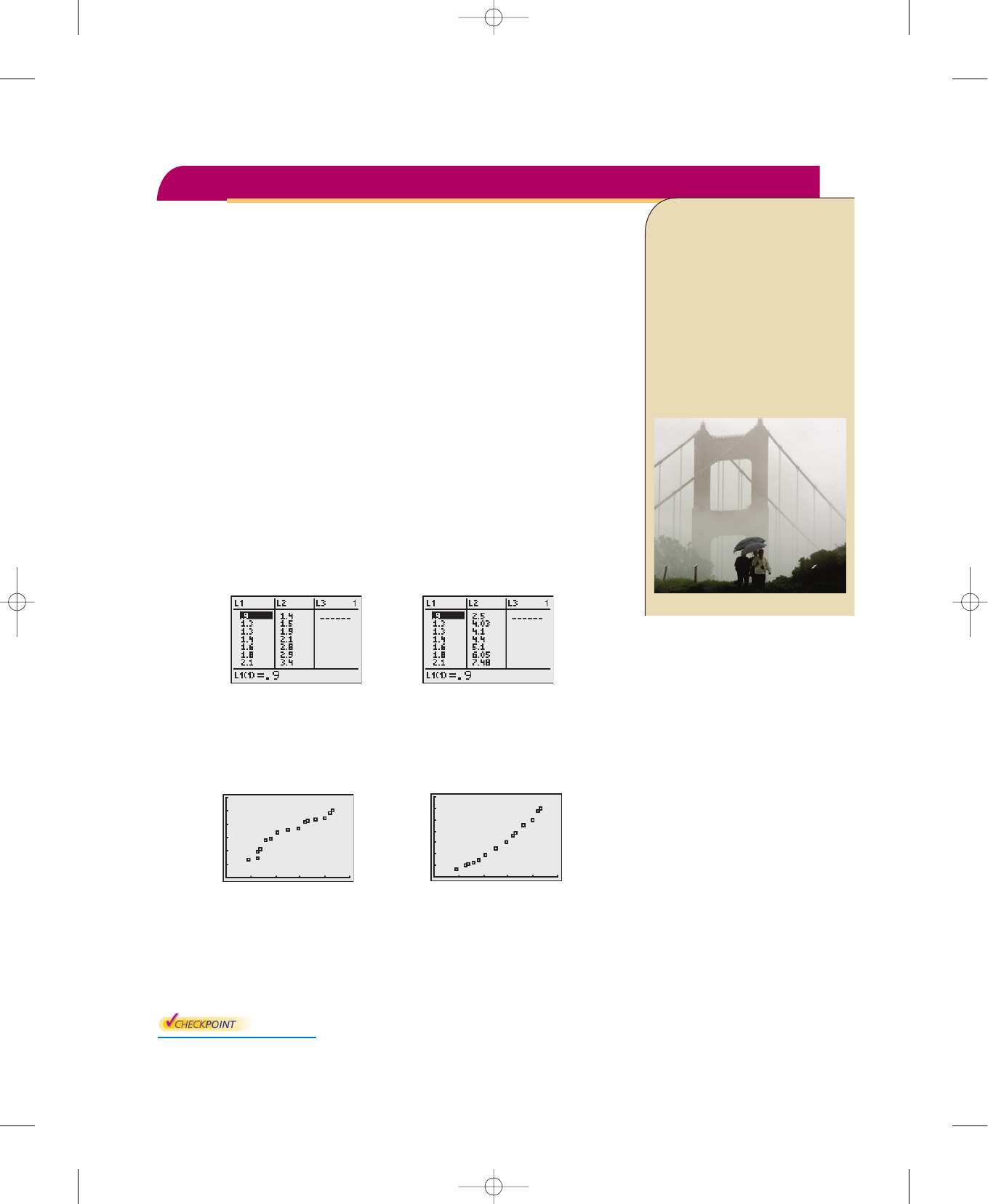
Many real-life situations can be modeled by

quadratic equations.For instance,in Exercise

15 on page 321,a quadratic equation is used

to model the monthly precipitation for

San Francisco,California.

Justin Sullivan/Getty Images

Section 3.7 Quadratic Models 317

Classifying Scatter Plots

In real life, many relationships between two variables are parabolic, as in Section

3.1, Example 5. A scatter plot can be used to give you an idea of which type of

model will best fit a set of data.

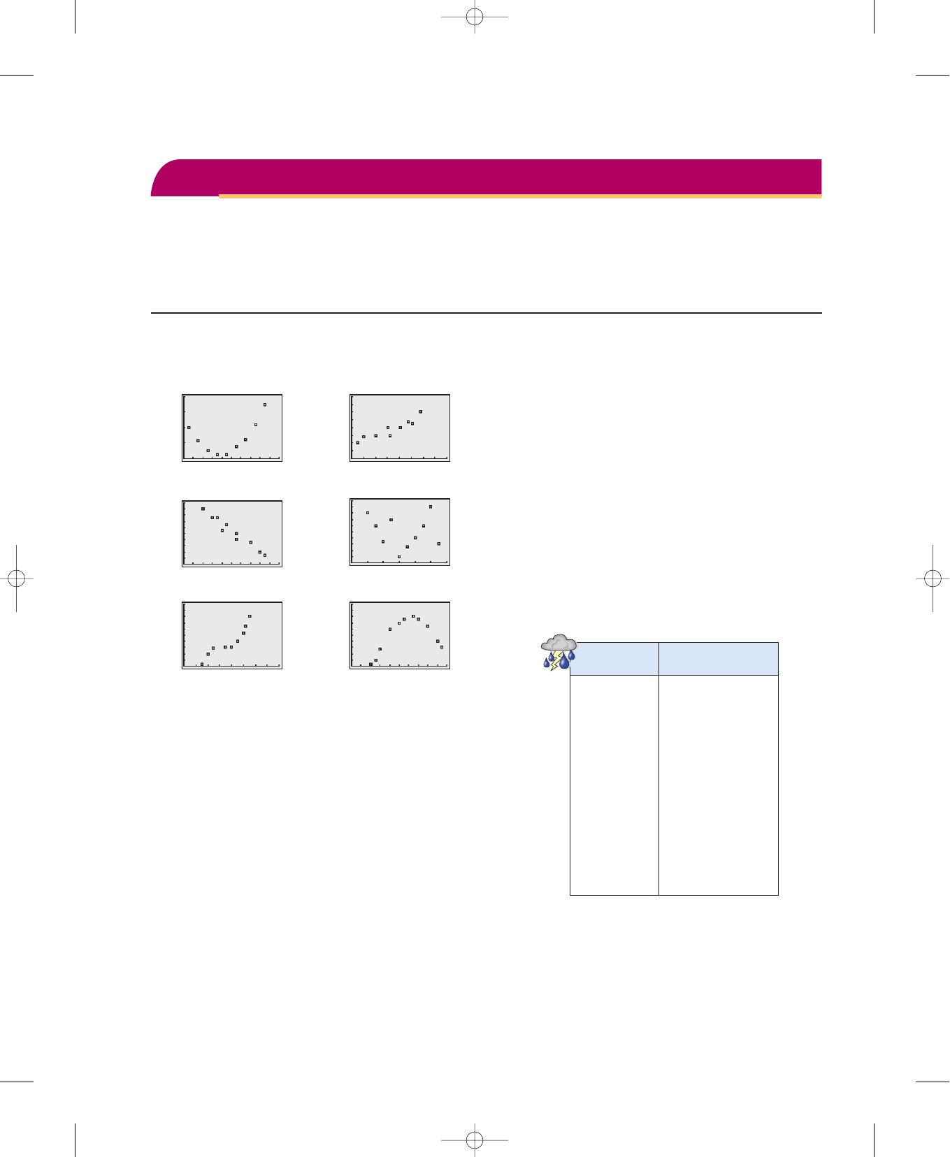
Example 1 Classifying Scatter Plots

Decide whether each set of data could be better modeled by a linear model,

or a quadratic model,

Solution

Begin by entering the data into a graphing utility, as shown in Figure 3.62.

(a) (b)

Figure 3.62

Then display the scatter plots, as shown in Figure 3.63.

(a) (b)

Figure 3.63

From the scatter plots, it appears that the data in part (a) follow a linear pattern.

So, it can be better modeled by a linear function. The data in part (b) follow a

parabolic pattern. So, it can be better modeled by a quadratic function.

Now try Exercise 3.

共

4.3, 23.9

兲共

4.2, 23.0

兲

共

4.0, 19.9

兲

共

3.6, 18.1

兲

共

3.3, 15.2

兲

共

3.2, 14.3

兲

共

2.9, 12.4

兲

共

2.5, 9.8

兲

共

2.1, 7.6

兲

共

2.1, 7.48

兲

共

1.8, 6.05

兲

共

1.6, 5.1

兲

共

1.4, 4.4

兲

共

1.3, 4.1

兲

共

1.3, 4.03

兲

共

0.9, 2.5

兲

共

4.3, 5.0

兲共

4.2, 4.8

兲

共

4.0, 4.5

兲

共

3.6, 4.4

兲

共

3.3, 4.3

兲

共

3.2, 4.2

兲

共

2.9, 3.7

兲

共

2.5, 3.6

兲

共

2.1, 3.4

兲

共

2.1, 3.4

兲

共

1.8, 2.9

兲

共

1.6, 2.8

兲

共

1.4, 2.1

兲

共

1.3, 1.9

兲

共

1.3, 1.5

兲

共

0.9, 1.4

兲

y ⫽ ax

⫹ bx ⫹ c.y ⫽ ax ⫹ b,

333371_0307.qxp 12/27/06 1:33 PM Page 317

318 Chapter 3 Polynomial and Rational Functions

080

y = −0.0082x

+ 0.746x + 13.47

For instructions on how to use the regression

feature, see Appendix A; for specific keystrokes, go to this textbook’s Online

Study Center.

TECHNOLOGY S U P P O R T

Fitting a Quadratic Model to Data

In Section 2.7, you created scatter plots of data and used a graphing utility to find

the least squares regression lines for the data. You can use a similar procedure to

find a model for nonlinear data. Once you have used a scatter plot to determine

the type of model that would best fit a set of data, there are several ways that you

can actually find the model. Each method is best used with a computer or

calculator, rather than with hand calculations.

Example 2 Fitting a Quadratic Model to Data

A study was done to compare the speed x (in miles per hour) with the mileage y

(in miles per gallon) of an automobile. The results are shown in the table.

(Source: Federal Highway Administration)

a. Use a graphing utility to create a scatter plot of the data.

b. Use the regression feature of the graphing utility to find a model that best fits

the data.

c. Approximate the speed at which the mileage is the greatest.

Solution

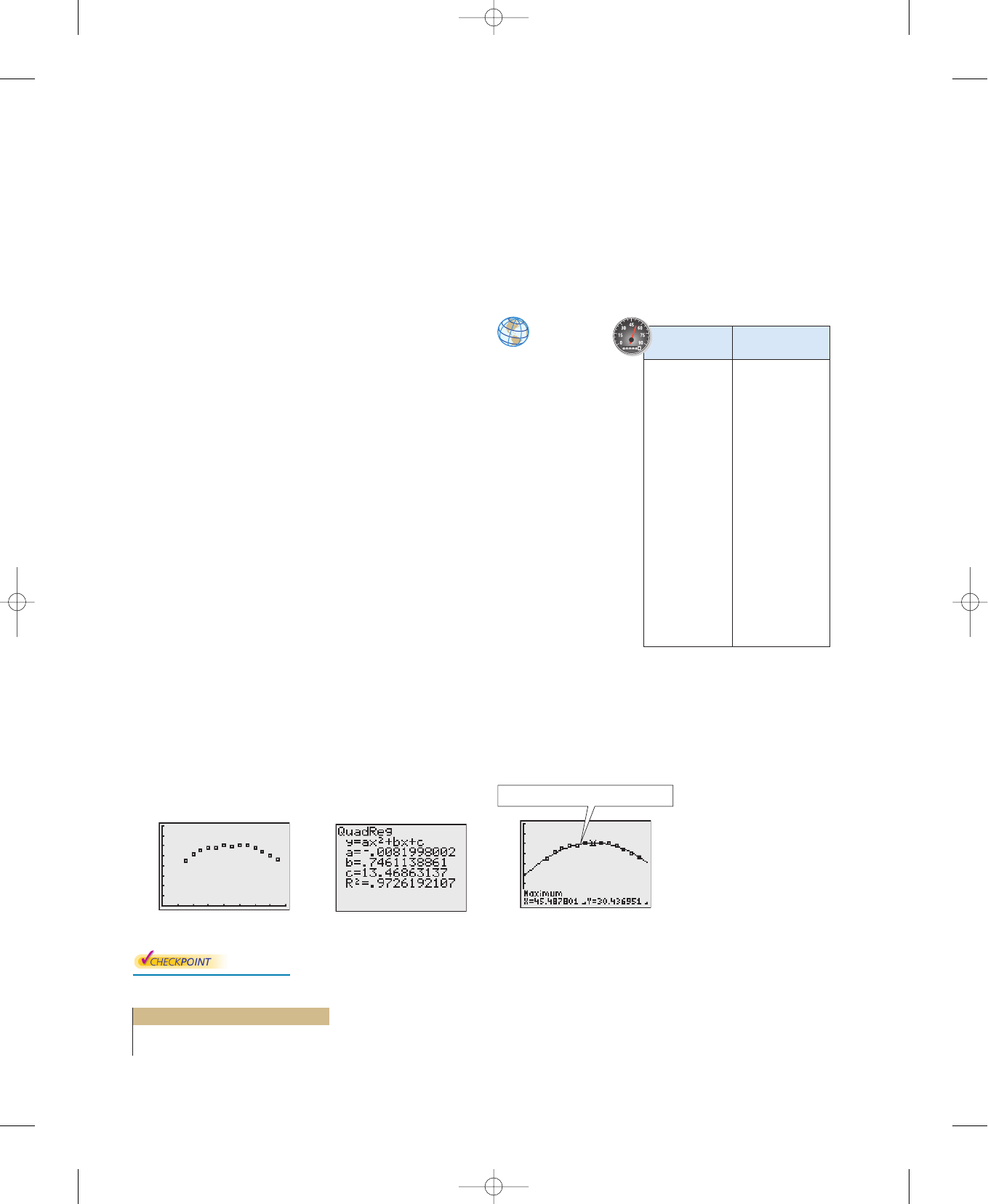
a. Begin by entering the data into a graphing utility and displaying the scatter

plot, as shown in Figure 3.64. From the scatter plot, you can see that the data

appears to follow a parabolic pattern.

b. Using the regression feature of a graphing utility, you can find the quadratic

model, as shown in Figure 3.65. So, the quadratic equation that best fits the

data is given by

Quadratic model

c. Graph the data and the model in the same viewing window, as shown in Figure

3.66. Use the maximum feature or the zoom and trace features of the graphing

utility to approximate the speed at which the mileage is greatest. You should

obtain a maximum of approximately as shown in Figure 3.66. So, the

speed at which the mileage is greatest is about 47 miles per hour.

Figure 3.64 Figure 3.65 Figure 3.66

Now try Exercise 15.

080

共

45, 30

兲

y ⫽⫺0.0082x

⫹ 0.746x ⫹ 13.47.

Speed, x Mileage, y

15 22.3

20 25.5

25 27.5

30 29.0

35 28.8

40 30.0

45 29.9

50 30.2

55 30.4

60 28.8

65 27.4

70 25.3

75 23.3

333371_0307.qxp 12/27/06 1:33 PM Page 318

Section 3.7 Quadratic Models 319

Example 3 Fitting a Quadratic Model to Data

A basketball is dropped from a height of about 5.25 feet. The height of the

basketball is recorded 23 times at intervals of about 0.02 second.* The results are

shown in the table. Use a graphing utility to find a model that best fits the data.

Then use the model to predict the time when the basketball will hit the ground.

Solution

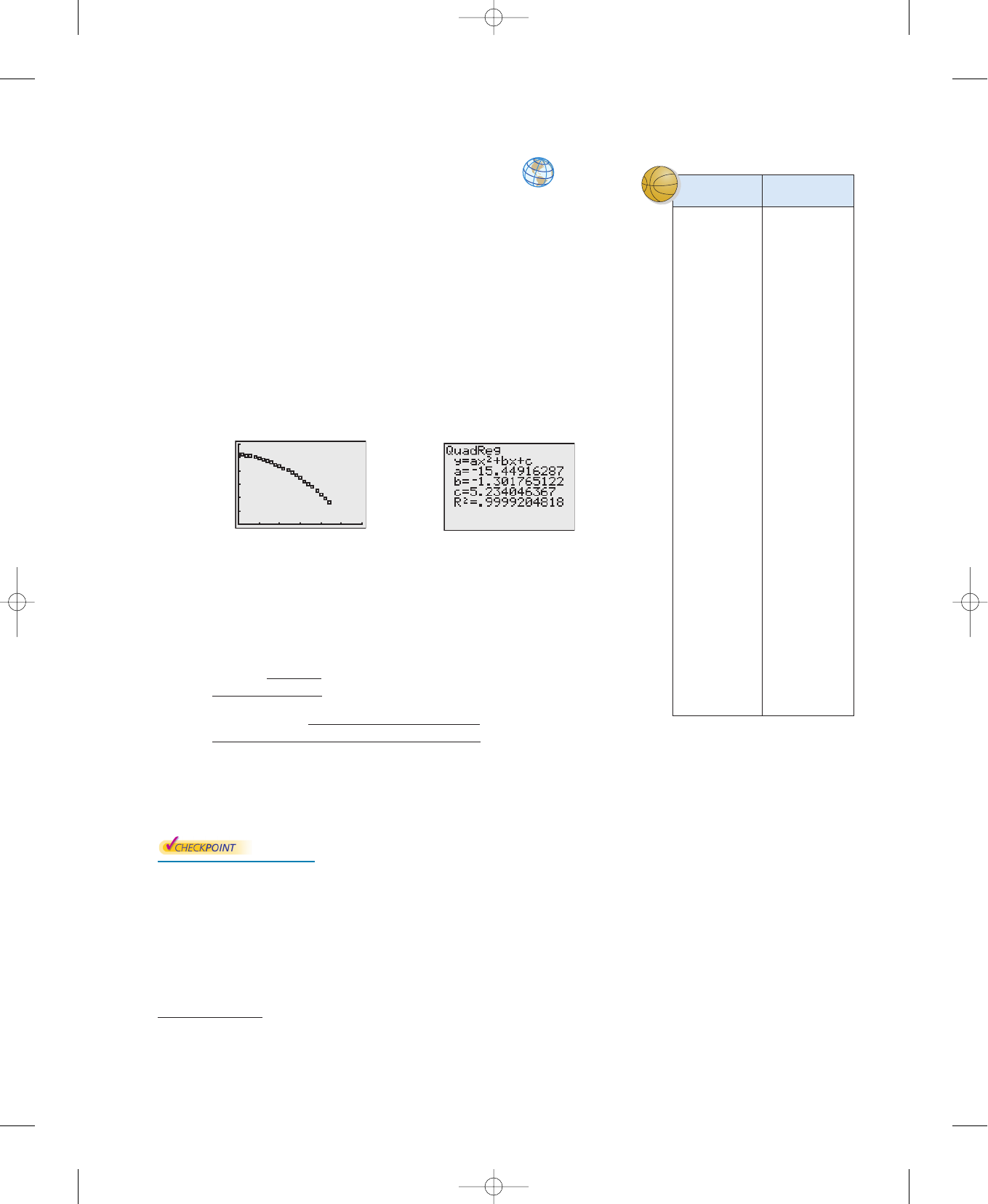
Begin by entering the data into a graphing utility and displaying the scatter plot,

as shown in Figure 3.67. From the scatter plot, you can see that the data has a

parabolic trend. So, using the regression feature of the graphing utility, you can

find the quadratic model, as shown in Figure 3.68. The quadratic model that best

fits the data is given by

Quadratic model

Figure 3.67 Figure 3.68

Using this model, you can predict the time when the basketball will hit the ground

by substituting 0 for y and solving the resulting equation for x.

Write original model.

Substitute 0 for y.

Quadratic Formula

Substitute for a, b, and c.

Choose positive solution.

So, the solution is about 0.54 second. In other words, the basketball will continue

to fall for about second more before hitting the ground.

Now try Exercise 17.

0.54 ⫺ 0.44 ⫽ 0.1

⬇ 0.54

⫽

⫺

共

⫺1.30

兲

冪

共

⫺1.30

兲

⫺ 4

共

⫺15.449

兲共

5.2

兲

共

⫺15.449

兲

x ⫽

⫺b

冪

⫺ 4ac

0 ⫽⫺15.449x

⫺ 1.30x ⫹ 5.2

y ⫽⫺15.449x

⫺ 1.30x ⫹ 5.2

0 0.6

y ⫽⫺15.449x

⫺ 1.30x ⫹ 5.2.

Choosing a Model

Sometimes it is not easy to distinguish from a scatter plot which type of model

will best fit the data. You should first find several models for the data, using the

Library of Parent Functions, and then choose the model that best fits the data by

comparing the y-values of each model with the actual y-values.

*Data was collected with a Texas Instruments CBL (Calculator-Based Laboratory) System.

Time, x Height, y

0.0 5.23594

0.02 5.20353

0.04 5.16031

0.06 5.09910

0.08 5.02707

0.099996 4.95146

0.119996 4.85062

0.139992 4.74979

0.159988 4.63096

0.179988 4.50132

0.199984 4.35728

0.219984 4.19523

0.23998 4.02958

0.25993 3.84593

0.27998 3.65507

0.299976 3.44981

0.319972 3.23375

0.339961 3.01048

0.359961 2.76921

0.379951 2.52074

0.399941 2.25786

0.419941 1.98058

0.439941 1.63488

333371_0307.qxp 12/27/06 1:33 PM Page 319

320 Chapter 3 Polynomial and Rational Functions

TECHNOLOGY TIP

When you use the regression feature of a graphing

utility, the program may output an “ -value.” This -value is the coefficient

of determination of the data and gives a measure of how well the model fits

the data. The coefficient of determination for the linear model in Example 4 is

and the coefficient of determination for the quadratic model is

Because the coefficient of determination for the quadratic model

is closer to 1, the quadratic model better fits the data.

⬇ 0.99456.

⬇ 0.97629

Example 4 Choosing a Model

The table shows the amounts y (in billions of dollars) spent on admission to

movie theaters in the United States for the years 1997 to 2003. Use the regression

feature of a graphing utility to find a linear model and a quadratic model for the

data. Determine which model better fits the data. (Source: U.S. Bureau of

Economic Analysis)

Solution

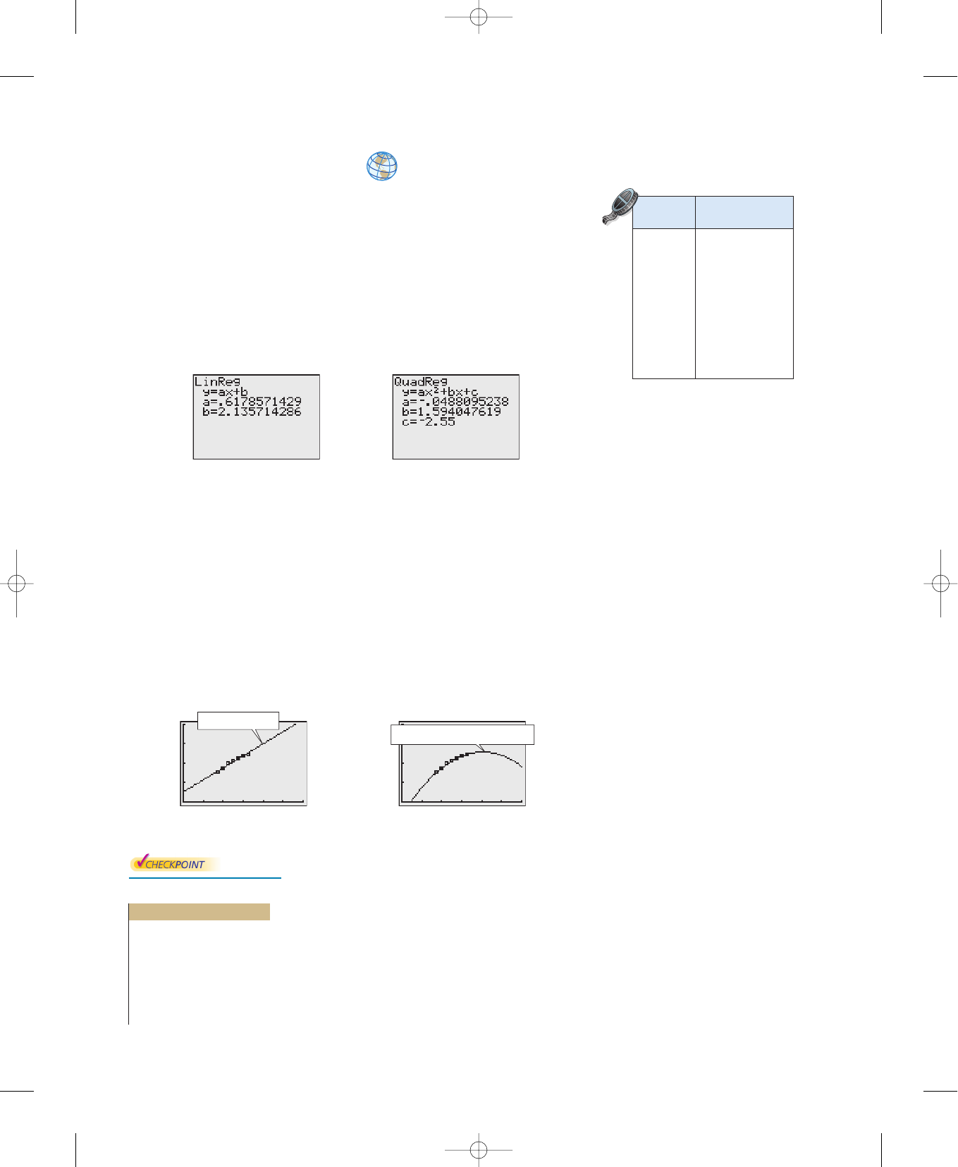
Let x represent the year, with corresponding to 1997. Begin by entering the

data into the graphing utility. Then use the regression feature to find a linear

model (see Figure 3.69) and a quadratic model (see Figure 3.70) for the data.

Figure 3.69 Linear Model Figure 3.70 Quadratic Model

So, a linear model for the data is given by

Linear model

and a quadratic model for the data is given by

Quadratic model

Plot the data and the linear model in the same viewing window, as shown

in Figure 3.71. Then plot the data and the quadratic model in the same viewing

window, as shown in Figure 3.72. To determine which model fits the data better,

compare the y-values given by each model with the actual y-values. The model

whose y-values are closest to the actual values is the better fit. In this case, the

better-fitting model is the quadratic model.

Figure 3.71 Figure 3.72

Now try Exercise 18.

024

y = − 0.049x

+ 1.59x − 2.6

024

y = 0.62x + 2.1

y ⫽⫺0.049x

⫹ 1.59x ⫺ 2.6.

y ⫽ 0.62x ⫹ 2.1

x ⫽ 7

Yea r Amount, y

1997 6.3

1998 6.9

1999 7.9

2000 8.6

2001 9.0

2002 9.6

2003 9.9

333371_0307.qxp 12/27/06 1:33 PM Page 320

Section 3.7 Quadratic Models 321

In Exercises 1–6, determine whether the scatter plot could

best be modeled by a linear model, a quadratic model, or

neither.

1. 2.

3. 4.

5. 6.

In Exercises 7–10, (a) use a graphing utility to create a

scatter plot of the data, (b) determine whether the data

could be better modeled by a linear model or a quadratic

model, (c) use the regression feature of a graphing utility to

find a model for the data, (d) use a graphing utility to graph

the model with the scatter plot from part (a), and (e) create

a table comparing the original data with the data given by

the model.

10.

In Exercises 11–14, (a) use the regression feature of a

graphing utility to find a linear model and a quadratic

model for the data, (b) determine the coefficient of determi-

nation for each model, and (c) use the coefficient of

determination to determine which model fits the data better.

11.

12.

13.

14.

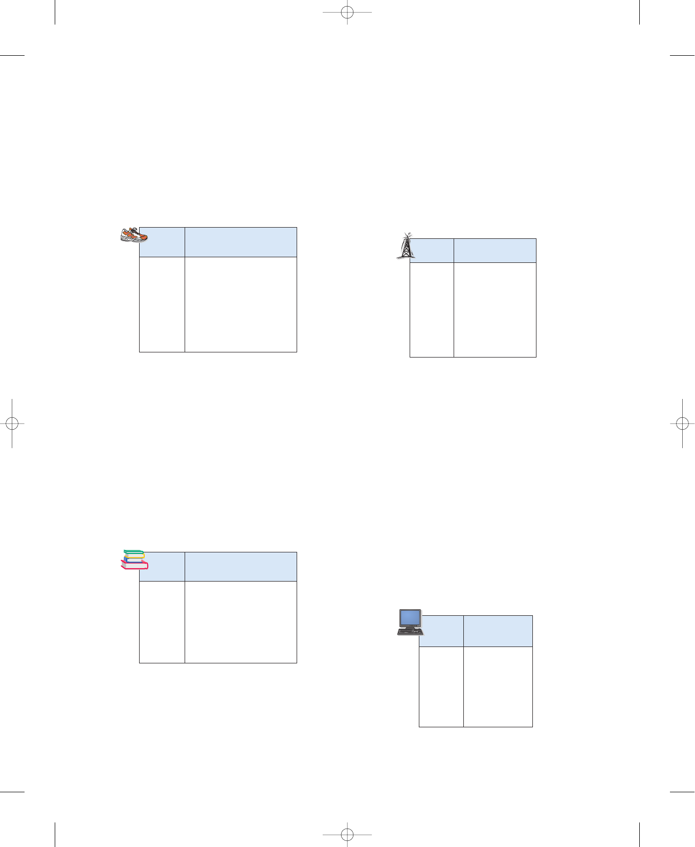
15. Meteorology The table shows the monthly normal

precipitation P (in inches) for San Francisco, California.

(Source: U.S. National Oceanic and Atmospheric

Administration)

(a) Use a graphing utility to create a scatter plot of the

data. Let t represent the month, with

corresponding to January.

(b) Use the regression feature of a graphing utility to find

a quadratic model for the data.

t ⫽ 1

共

25, 430

兲共

20, 436

兲

共

15, 478

兲

共

10, 512

兲

共

5, 551

兲

共

0, 587

兲

共

⫺5, 653

兲

共

⫺10, 704

兲

共

⫺15, 744

兲

共

⫺20, 805

兲

共

12, ⫺5.3

兲共

10, ⫺3.6

兲

共

8, ⫺1.8

兲

共

6, ⫺0.1

兲

共

4, 1.7

兲

共

2, 3.5

兲

共

0, 5.4

兲

共

⫺2, 7.0

兲

共

⫺4, 9.0

兲

共

⫺6, 10.7

兲

共

9, 19.0

兲共

8, 16.8

兲

共

7, 14.5

兲

共

6, 12.6

兲

共

5, 10.5

兲

共

4, 8.3

兲

共

3, 6.3

兲

共

2, 4.1

兲

共

1, 2.0

兲

共

0, 0.1

兲

共

10, 27.1

兲共

9, 24.0

兲

共

8, 20.1

兲

共

7, 17.5

兲

共

6, 15.0

兲

共

5, 13.9

兲

共

4, 10.6

兲

共

3, 8.8

兲

共

2, 6.5

兲

共

1, 4.0

兲

共

22, 5325

兲共

20, 6125

兲

共

18, 6820

兲

共

16, 7325

兲

共

14, 7700

兲

共

12, 7975

兲

共

10, 7590

兲

共

8, 7915

兲

共

6, 7710

兲

共

4, 7335

兲

共

2, 6815

兲

共

0, 6140

兲

共

55, 5010

兲共

50, 3500

兲

共

45, 2225

兲

共

40, 1275

兲

共

35, 575

兲

共

30, 145

兲

共

25, 12

兲

共

20, 150

兲

共

15, 565

兲

共

10, 1250

兲

共

5, 2235

兲

共

0, 3480

兲

共

8, 9.0

兲共

7, 9.2

兲

共

6, 9.4

兲

共

5, 9.4

兲

共

4, 9.6

兲

共

3, 9.9

兲

共

2, 10.1

兲

共

1, 10.3

兲

共

0, 10.4

兲

共

⫺1, 10.7

兲

共

⫺2, 11.0

兲

共

10, 3.6

兲共

9, 3.5

兲

共

8, 3.4

兲

共

7, 3.2

兲

共

6, 3.0

兲

共

5, 3.0

兲

共

4, 2.9

兲

共

3, 2.8

兲

共

2, 2.5

兲

共

1, 2.4

兲

共

0, 2.1

兲

010

020

3.7 Exercises See www.CalcChat.com for worked-out solutions to odd-numbered exercises.

Vocabulary Check

Fill in the blanks.

1. A scatter plot with either a positive or a negative correlation can be better modeled by a _______ equation.

2. A scatter plot that appears parabolic can be better modeled by a _______ equation.

Month Precipitation, P

January 4.45

February 4.01

March 3.26

April 1.17

May 0.38

June 0.11

July 0.03

August 0.07

September 0.20

October 1.40

November 2.49

December 2.89

333371_0307.qxp 12/27/06 1:33 PM Page 321

322 Chapter 3 Polynomial and Rational Functions

ter plot from part (a).

(d) Use the graph from part (c) to determine in which

month the normal precipitation in San Francisco is the

least.

16. Sales The table shows the sales S (in millions of dollars)

for jogging and running shoes from 1998 to 2004.

(Source: National Sporting Goods Association)

(a) Use a graphing utility to create a scatter plot of the

data. Let t represent the year, with corresponding

to 1998.

(b) Use the regression feature of a graphing utility to find

a quadratic model for the data.

scatter plot from part (a).

(d) Use the model to find when sales of jogging and

running shoes will exceed 2 billion dollars.

(e) Is this a good model for predicting future sales?

Explain.

17. Sales The table shows college textbook sales (in

millions of dollars) in the United States from 2000 to 2005.

(Source: Book Industry Study Group, Inc.)

(a) Use a graphing utility to create a scatter plot of the

data. Let t represent the year, with corresponding

to 2000.

(b) Use the regression feature of a graphing utility to find

a quadratic model for the data.

scatter plot from part (a).

(d) Use the model to find when the sales of college

textbooks will exceed 10 billion dollars.

(e) Is this a good model for predicting future sales?

Explain.

18. Media The table shows the numbers S of FM radio

stations in the United States from 1997 to 2003. (Source:

Federal Communications Commission)

(a) Use a graphing utility to create a scatter plot of the

data. Let t represent the year, with corresponding

to 1997.

(b) Use the regression feature of a graphing utility to find

a linear model for the data and identify the coefficient

of determination.

scatter plot from part (a).

(d) Use the regression feature of a graphing utility to find

a quadratic model for the data and identify the coeffi-

cient of determination.

(e) Use a graphing utility to graph the quadratic model

with the scatter plot from part (a).

(f) Which model is a better fit for the data?

(g) Use each model to find when the number of FM

stations will exceed 7000.

19. Entertainment The table shows the amounts A (in dol-

lars) spent per person on the Internet in the United States

from 2000 to 2005. (Source: Veronis Suhler Stevenson)

t ⫽ 7

t ⫽ 0

t ⫽ 8

Yea r FM stations, S

1997 5542

1998 5662

1999 5766

2000 5892

2001 6051

2002 6161

2003 6207

Year

Amount, A

(in dollars)

2000 49.64

2001 68.94

2002 84.76

2003 96.35

2004 107.02

2005 117.72

Year

Sales, S

(in millions of dollars)

1998 1469

1999 1502

2000 1638

2001 1670

2002 1733

2003 1802

2004 1838

Year

Textbook sales, S

(in millions of dollars)

2000 4265.2

2001 4570.7

2002 4899.1

2003 5085.9

2004 5478.6

2005 5703.2

333371_0307.qxp 12/27/06 1:33 PM Page 322

Section 3.7 Quadratic Models 323

(a) Use a graphing utility to create a scatter plot of the

data. Let t represent the year, with corresponding

to 2000.

(b) A cubic model for the data is

which has an -value of

0.99992. Use a graphing utility to graph this model

with the scatter plot from part (a). Is the cubic model a

good fit for the data? Explain.

a quadratic model for the data and identify the coeffi-

cient of determination.

(d) Use a graphing utility to graph the quadratic model

with the scatter plot from part (a). Is the quadratic

model a good fit for the data? Explain.

(e) Which model is a better fit for the data? Explain.

(f) The projected amounts A* spent per person on the

Internet for the years 2006 to 2008 are shown in the

table. Use the models from parts (b) and (c) to predict

the amount spent for the same years. Explain why your

values may differ from those in the table.

20. Entertainment The table shows the amounts A (in hours)

of time per person spent watching television and movies,

listening to recorded music, playing video games, and

reading books and magazines in the United States from

2000 to 2005. (Source: Veronis Suhler Stevenson)

(a) Use a graphing utility to create a scatter plot of the

data. Let t represent the year, with corresponding

to 2000.

(b) A cubic model for the data is

which has an -value of

Use a graphing utility to graph this model

with the scatter plot from part (a). Is the cubic model a

good fit for the data? Explain.

a quadratic model for the data and identify the coeffi-

cient of determination.

(d) Use a graphing utility to graph the quadratic model

with the scatter plot from part (a). Is the quadratic

model a good fit for the data? Explain.

(e) Which model is a better fit for the data? Explain.

(f) The projected amounts A* of time spent per person for

the years 2006 to 2008 are shown in the table. Use the

models from parts (b) and (c) to predict the number of

hours for the same years. Explain why your values may

differ from those in the table.

Synthesis

True or False? In Exercises 21 and 22, determine whether

the statement is true or false. Justify your answer.

21. The graph of a quadratic model with a negative leading

coefficient will have a maximum value at its vertex.

22. The graph of a quadratic model with a positive leading

coefficient will have a minimum value at its vertex.

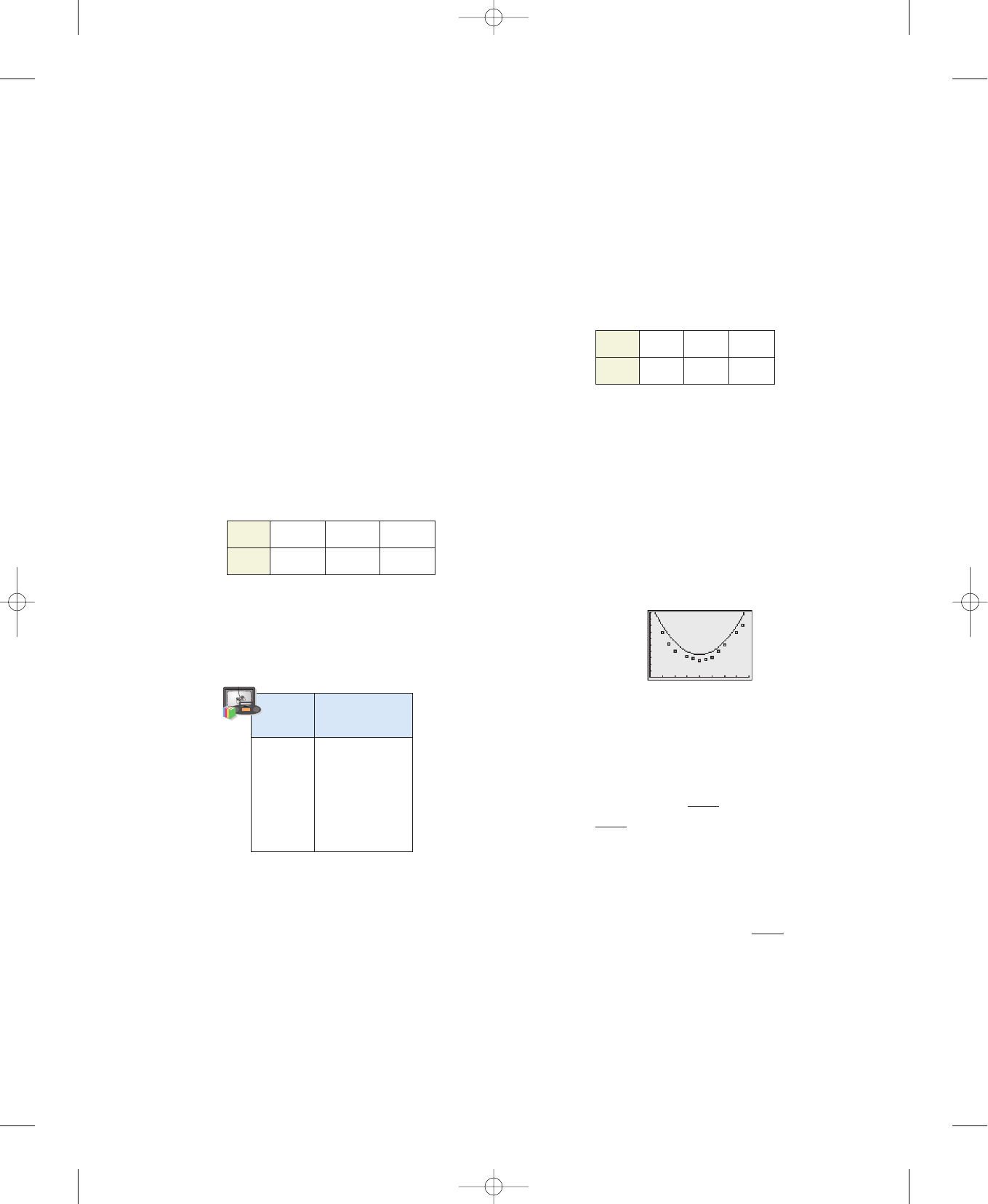
23. Writing Explain why the parabola shown in the figure is

not a good fit for the data.

Skills Review

In Exercises 24–27, find (a) and (b)

24.

25.

26.

27.

In Exercises 28–31, determine algebraically whether the

function is one-to-one. If it is, find its inverse function.

Verify your answer graphically.

28. 29.

30. 31.

In Exercises 32–35, plot the complex number in the complex

plane.

32.

33.

34. 35. 8i⫺5i

⫺2 ⫹ 4i1 ⫺ 3i

≥

共

兲

⫽ 2x

⫺ 3,x

≥

共

兲

⫽ x

⫹ 5,

共

兲

⫽

x ⫺ 4

共

兲

⫽ 2x ⫹ 5

共

兲

⫽ x

⫺ 5f

共

兲

⫽

冪

x ⫹ 5,

共

兲

⫽

冪

x ⫹ 1f

共

兲

⫽ x

⫺ 1,

共

兲

⫽ 2x

⫺ 1f

共

兲

⫽ 5x ⫹ 8,

共

兲

⫽ x

⫹ 3f

共

兲

⫽ 2x ⫺ 1,

⬚

f.f

⬚

0.99667.

13.61t

⫹ 33.2t ⫹ 3493

A ⫽

⫺

1.500t

⫹

t ⫽ 0

3.0440t

⫹ 22.485t ⫹ 49.55

S ⫽ 0.25444t

⫺

t ⫽ 0

Year 2006 2007 2008

127.76 140.15 154.29

Year 2006 2007 2008

3890 3949 4059

Year

Amount, A

(in hours)

2000 3492

2001 3540

2002 3606

2003 3663

2004 3757

2005 3809

DISC 1

TRACK 4

333371_0307.qxp 1/2/07 9:50 AM Page 323